Hi everybody,

this is the third and last entry about DTM 2020 Class One cars and will build on the previous two, focusing on a performance analysis based on lap time simulation. I will look into the sensitivity of a few key metrics to certain setup and design parameters and on how the team could optimize the usage on tracks of aids like the DRS.

Lap time simulation tool, track and vehicle model
For this study I used my lap time simulation tool. Anyway, I did this analysis some time ago, and the tool did not incorporate yet all the features it has now. I will post an entry on the latest additions I built into my lap time simulator: examples of features that the tool did not have yet at the time I performed this study were suspension compliance (camber stiffness), separation between sprung and unsprung masses, an improved rolling radius calculation and some new enhancements in track modeling.

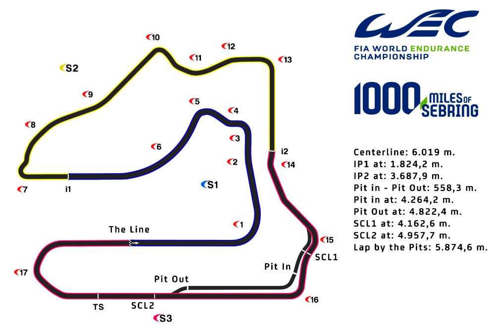
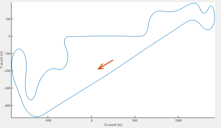
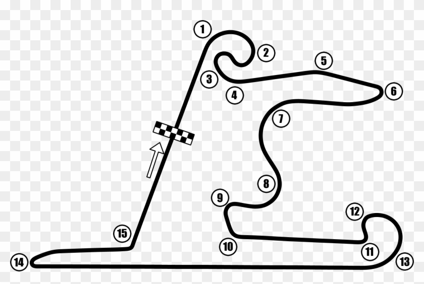
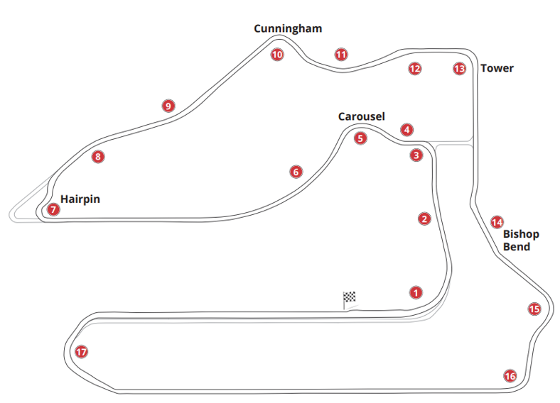
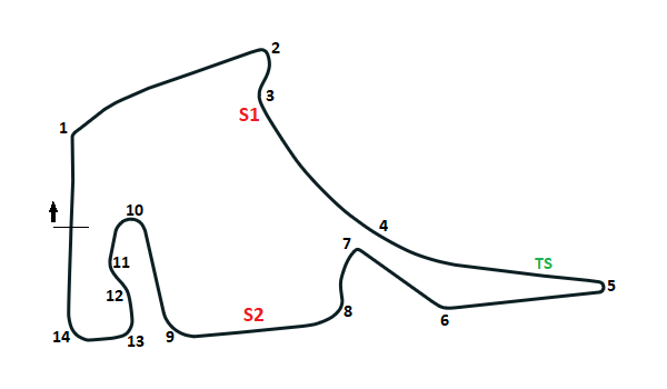
This study will focus on the Hockenheim circuit, in its GP configuration. Hockenheim is a 4.574 kilometer long, German track that historically belongs to DTM calendar and also offers an extremely interesting combination of slow, medium and high speed corners, together with a long, full throttle section, where pretty high top speeds can be achieved and where most of the overtaking maneuvers take place.
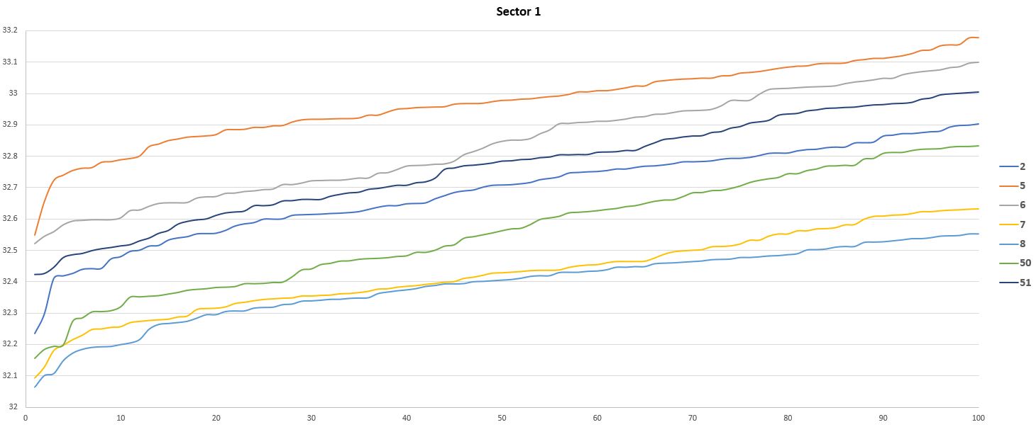
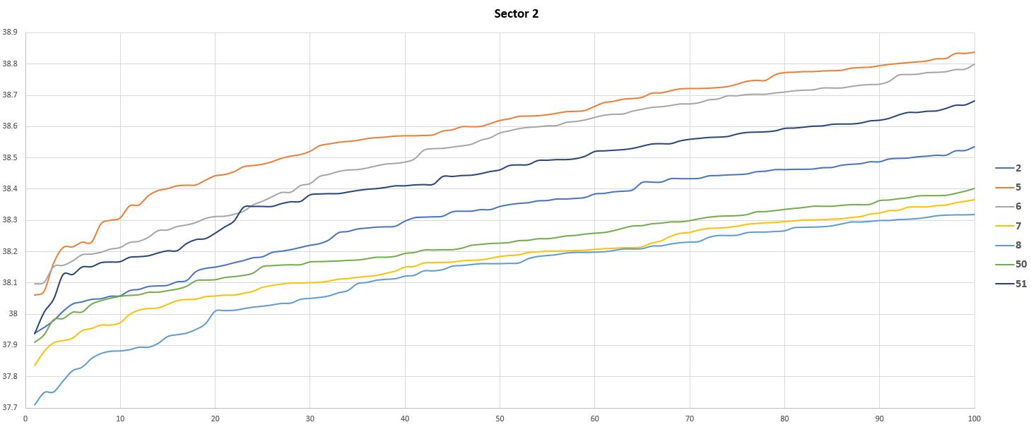
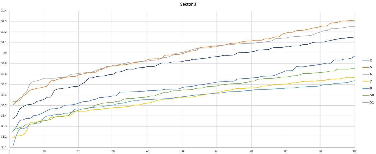
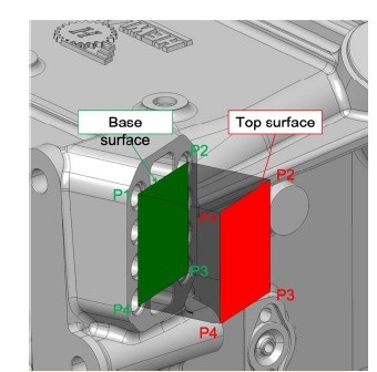
The circuit is usually divided into three sectors, as described in figure 1, that also shows the numbering for the corners this article will refer to.

Hockenheim circuit map with track sectors and corners numbers

The vehicle model was built basing on the data discussed in the two previous entries and referring to a hypothetical qualifying trim. A summary of its main features is:

• Vehicle mass of 1090 kg (1070 kg for car and driver, 20kg fuel)
• Wheelbase 2750 mm
• Front track width 1640 millimeter
• Rear track width 1610 millimeter
• Mass distribution of 50% on the front axle
• Brake balance 62% on the front axle
• Aeromap and average values of downforce and drag as described last month, aerodynamic balance of about 45.8% (averages on the map)
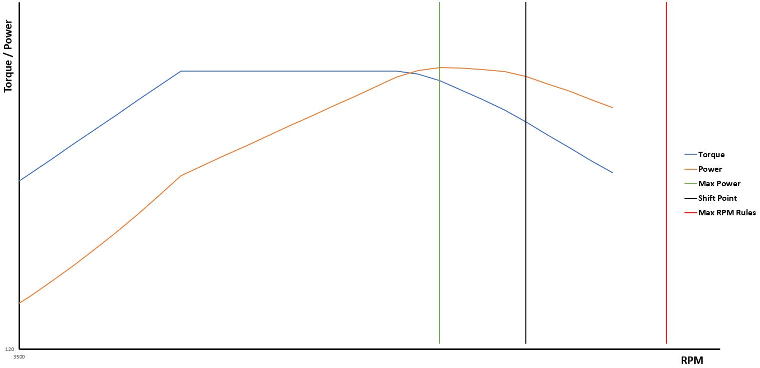
• Maximum engine power of about 615hp
• Gear ratios provided by the regulations, drop gears selected among allowed options
• DRS effect: drag drops about 18%, downforce by about 20%, aerodynamic balance moves significantly forward
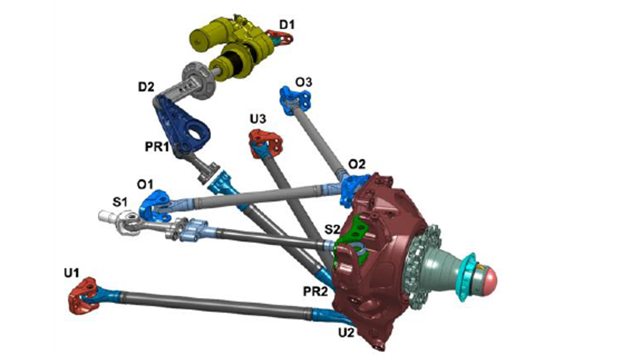
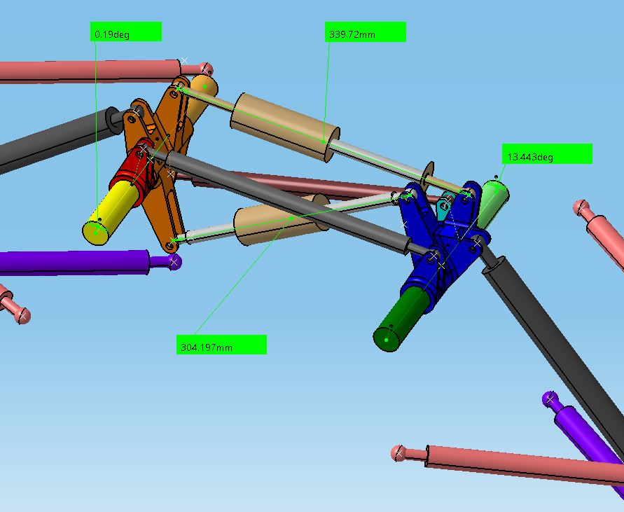
• Suspension kinematics based on manufacturers data
• Suspensions stiffness and static camber as described in previous instalment

First simulation run
The first simulation runs were performed without activating the DRS. I did not model the P2P, for the sake of simplicity. Moreover, its effect should be smaller than DRS one, because of the limited time it can be used.
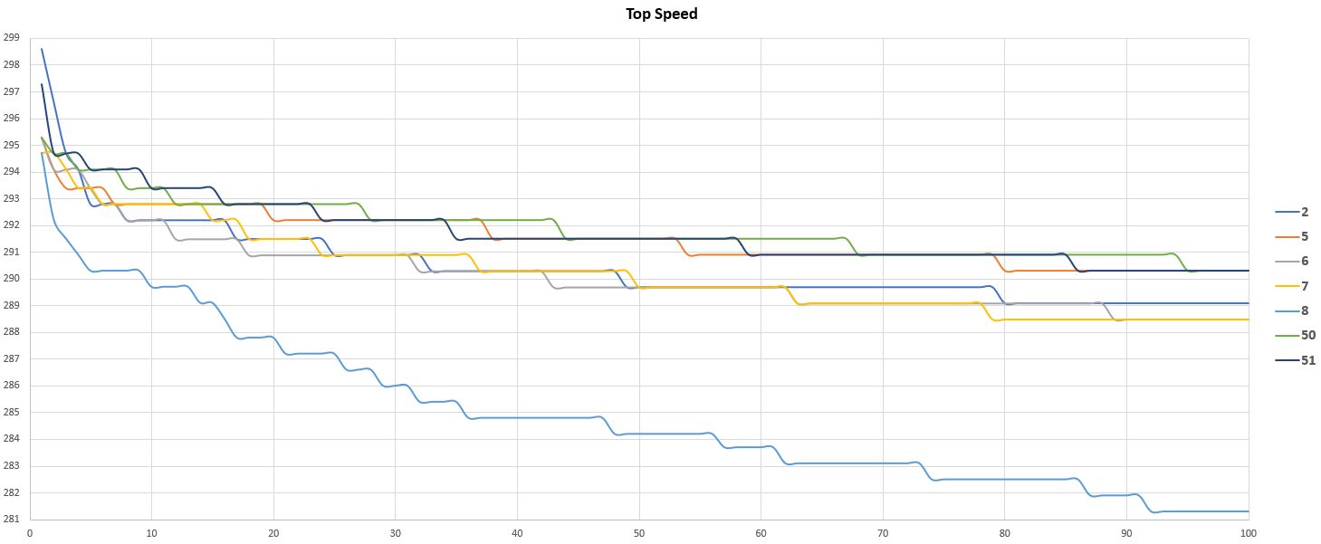
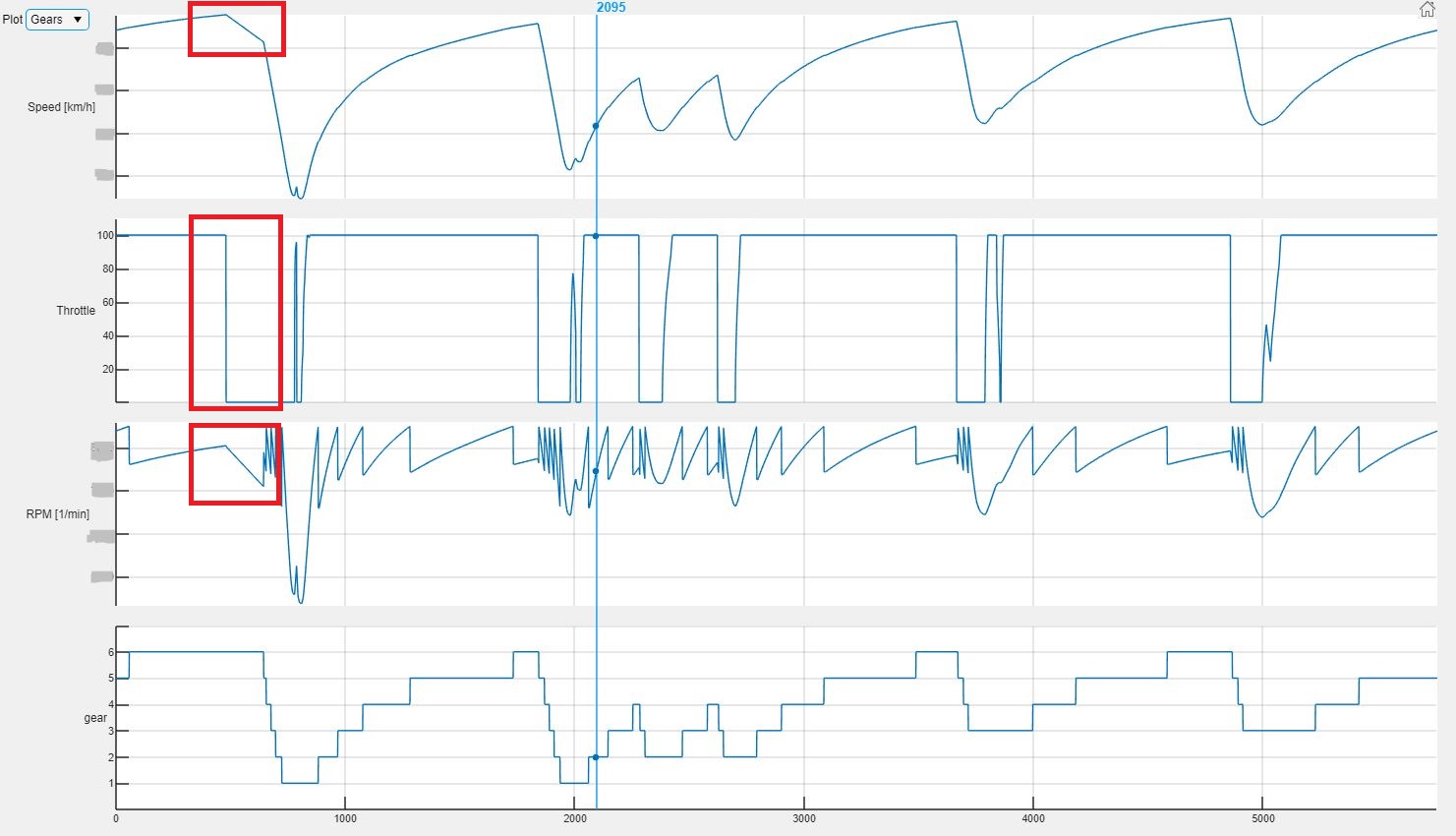
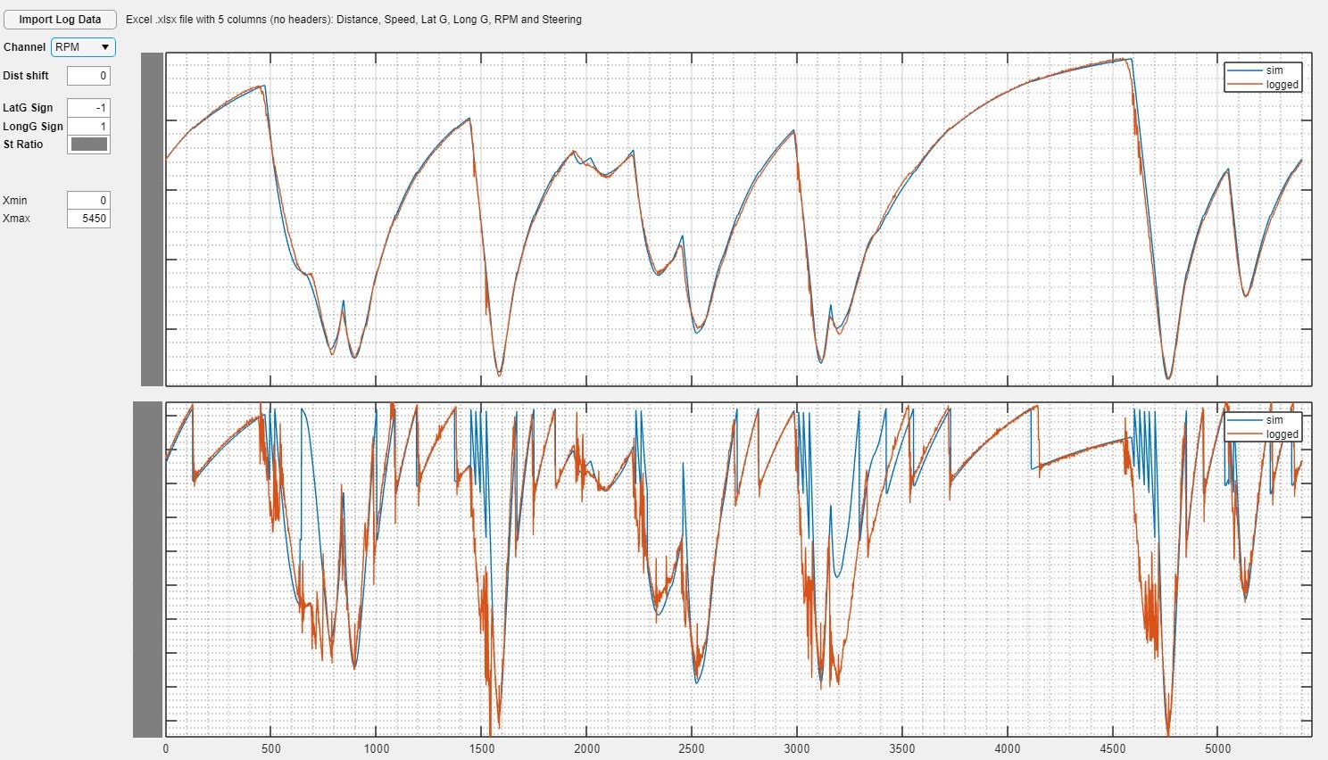
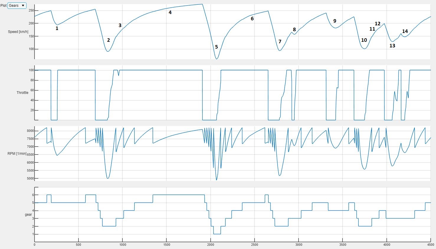
The first run produced a lap time of 1’28.885, with a top speed of 274.4 kph. The model achieves a maximum lateral acceleration of 2.6g in turn 1, with a minimum speed of about 193 kph. Turn 5 is the slowest corner and the only one where first gear is engaged; the minimum speed here is about 60 kph. Turn 2, turn 7 and turn 10 are also relatively slow corners, driven in second gear and with minimum speeds between 90 and 100 kph. Turn 9 is another fast bend: here our vehicle model pulls about 2.5g, with a minimum speed of about 181 kph.
Slightly less than 70% of the lap is covered with the throttle completely open.
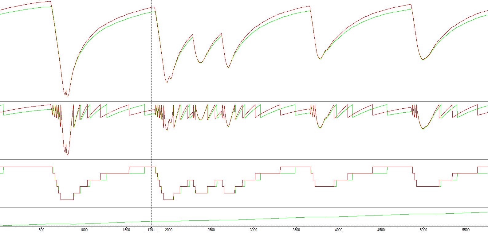
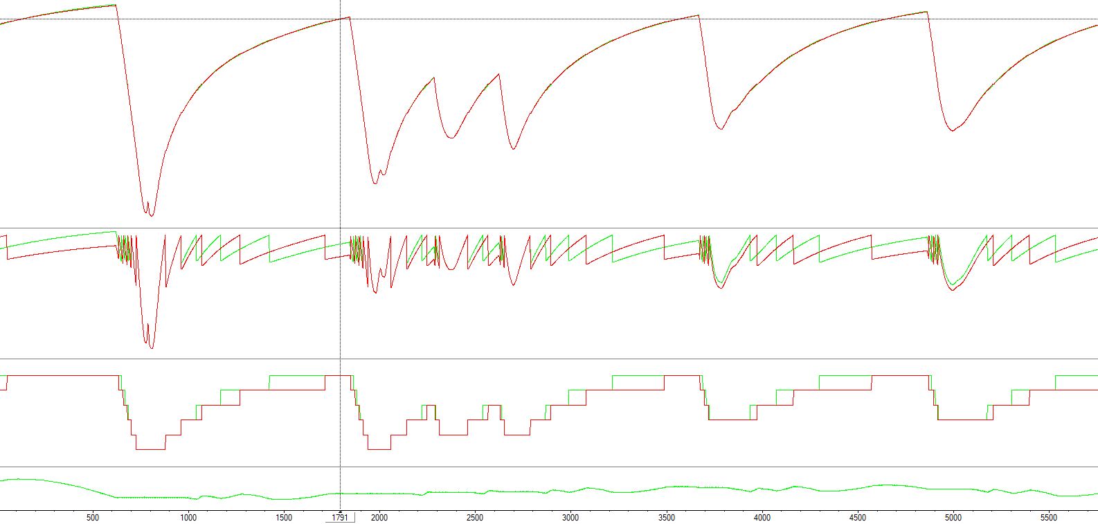
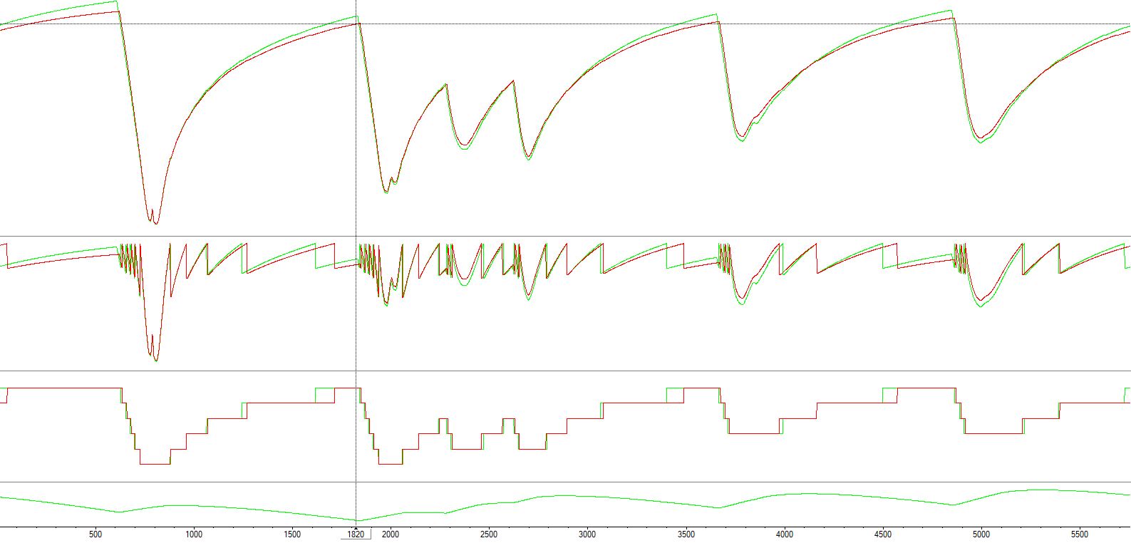
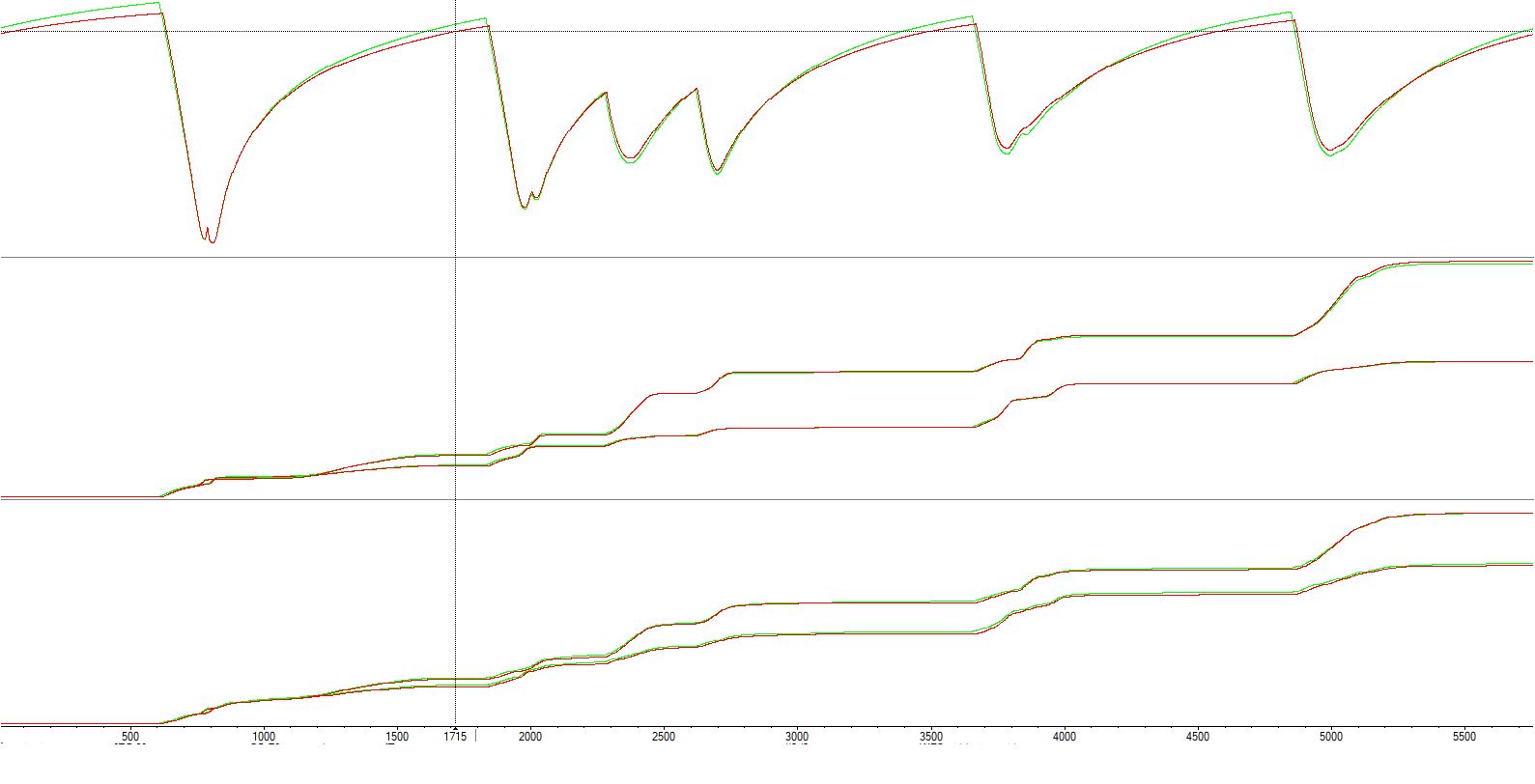
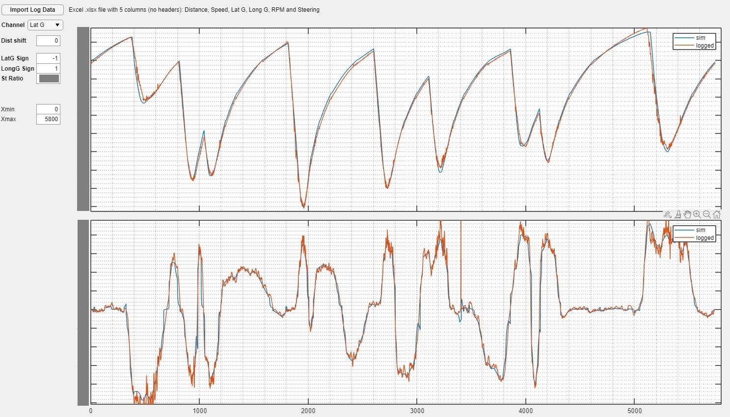
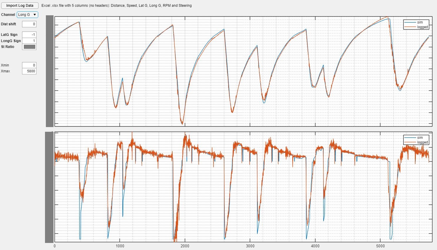
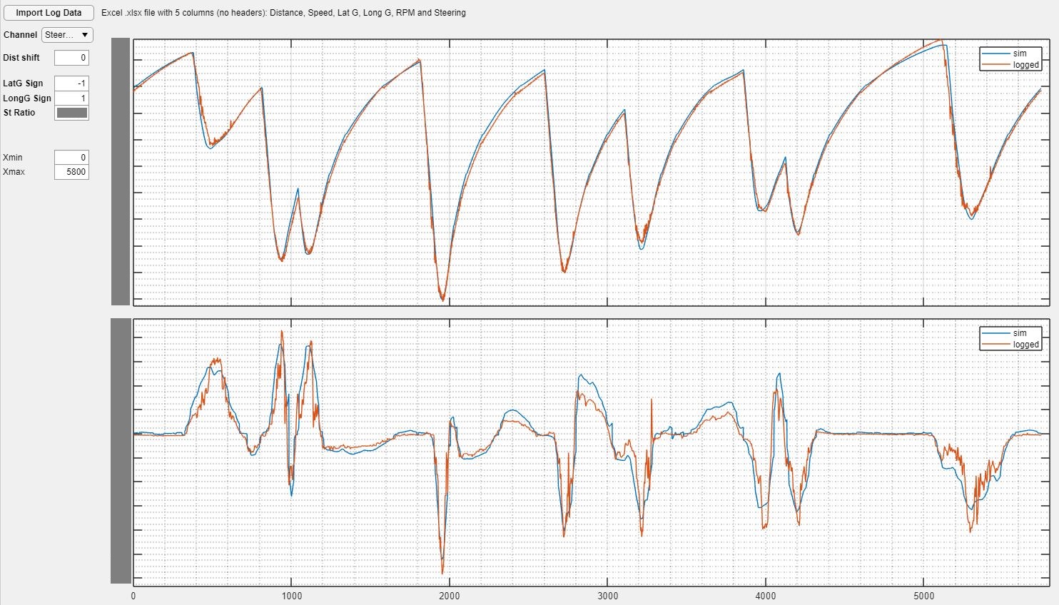
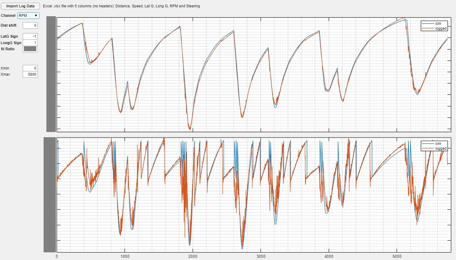
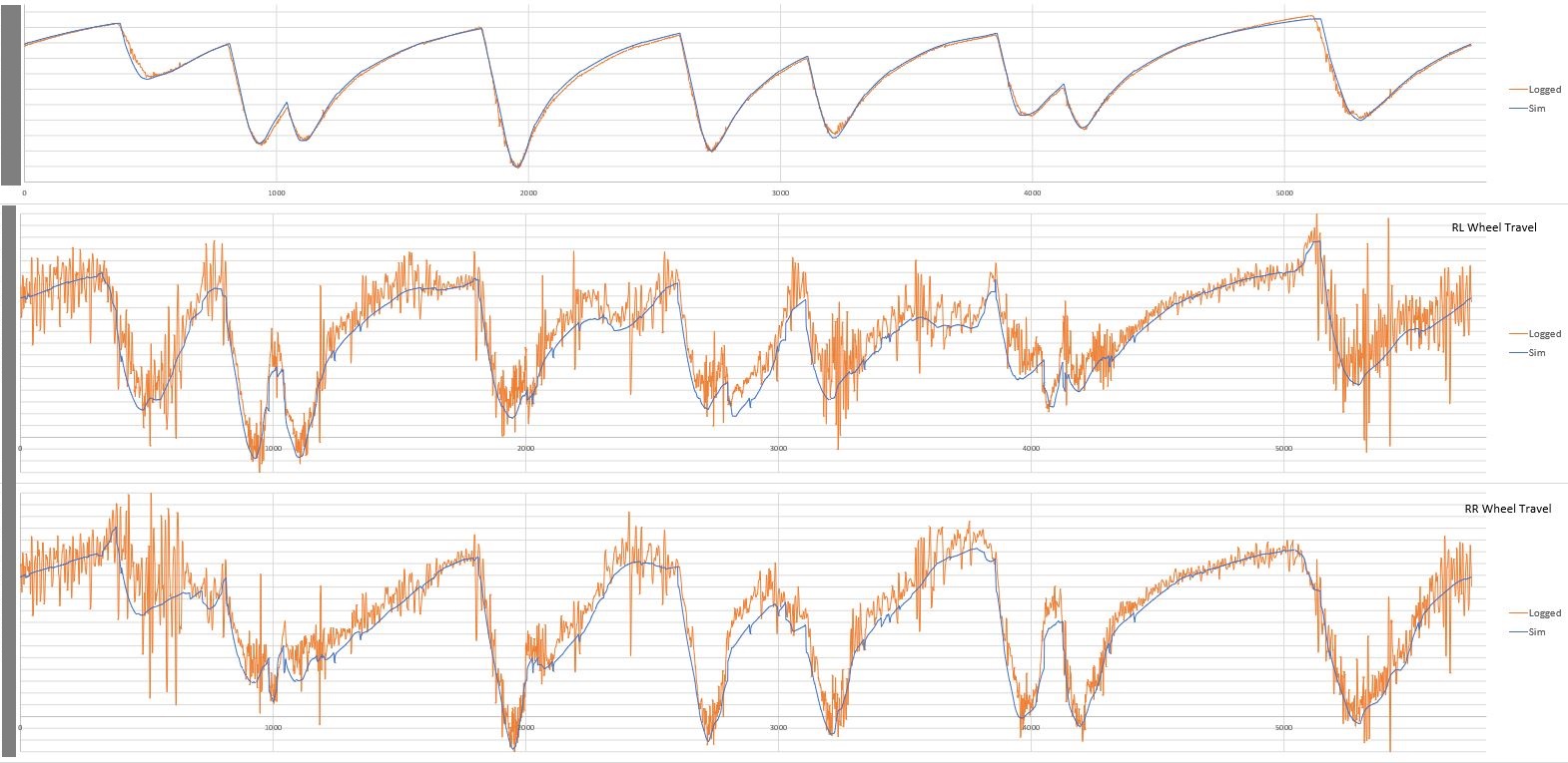
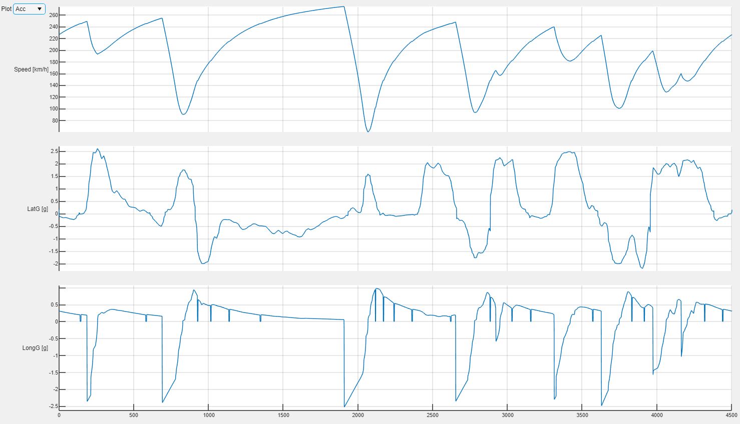
Figure 2 depicts, from above, the traces relative to vehicle’s speed, throttle position, RPM and engaged gears, while figure 3 shows again speed, lateral acceleration and longitudinal acceleration. Corners numbers are also shown in figure 2.

First simulation results. From above: speed, throttle position, RPM and engaged gear

First simulation results. From above: speed, lateral acceleration and longitudinal acceleration

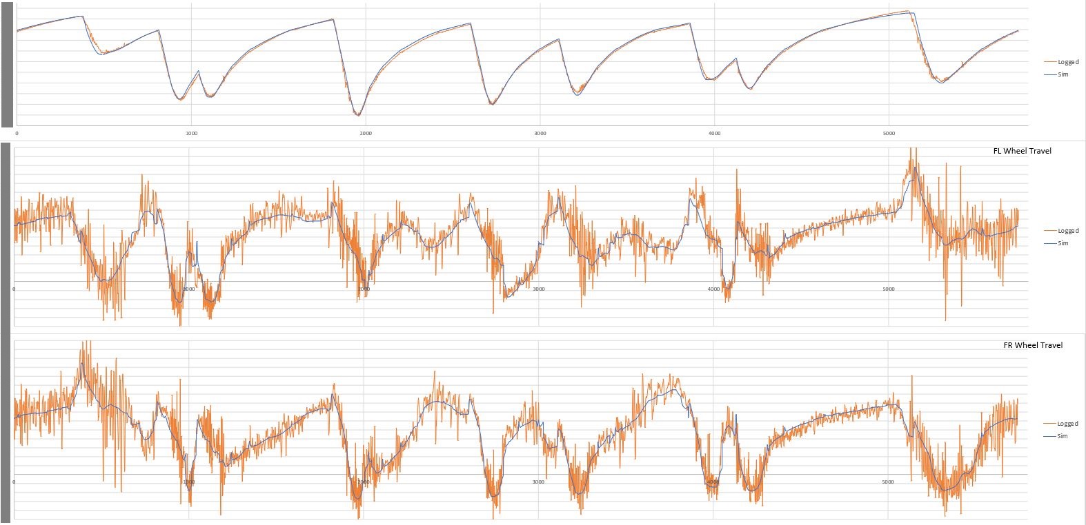
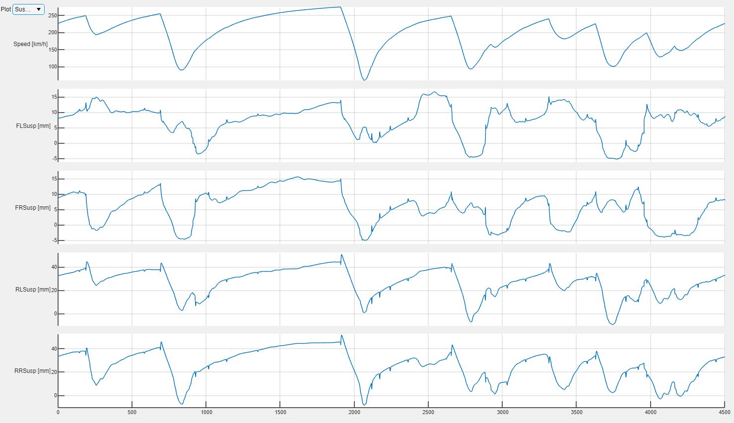
Suspensions’ behavior is particularly interesting. Wheel travels are shown in figure 4, where the first trace from above is car’s speed and the following ones are respectively front left, front right, rear left and rear right wheel travels. Positive values for those indicate the suspension moving into jounce (compressing the springs).
Front wheel travels are, as expected, much smaller than the rear ones, as front wheel rates in heave are much higher. Front dynamic ride heights have a critical influence on both downforce and aerodynamic balance.
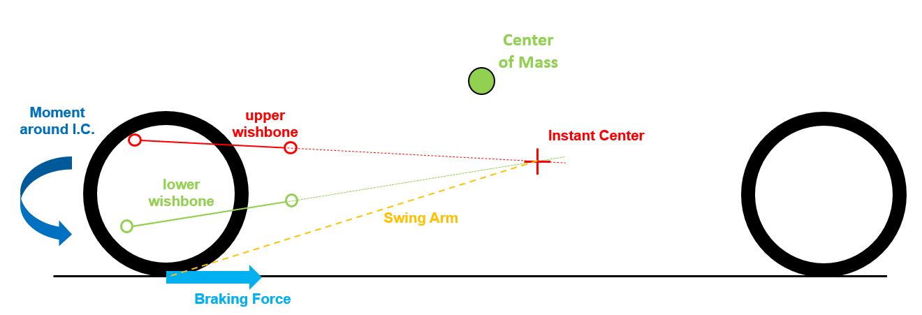
The front axle achieves the highest wheel travels in roll, not in heave or pitch (for example during a braking maneuver). Also, front springs initial compression during braking is minimal, despite the suspension not engaging any bump stop and the pretty high longitudinal acceleration. The low vertical wheel travel in braking is linked to the aggressive use of anti-dive effects at the front while the big wheel travels in roll are due to the relatively low front roll stiffness and the low geometrical anti roll effects (or, in other term, low roll center height), as described in part 2.
The situation is different at the rear, anyway. A first key element, is how the rear springs are compressed at the beginning of a braking phase, despite the longitudinal load transfer that tends to decrease the vertical load on the rear axle. Also very interesting, this counterintuitive phenomenon only happens at the very beginning of the braking zone; this is again a consequence of the high anti-effects designed into the suspension: because of the high longitudinal forces in the first part of a braking, a high moment that tend to extend the springs is generated.
Rear wheel travels in roll are, on the contrary with respect to the front, smaller than the travels that the rear axle experiences in heave. Indeed, the rear axle has a higher roll stiffness and the geometrical anti roll effects are also sensibly bigger than front ones (higher roll center).

First simulation results. From above: speed, front left, front right, rear left and rear right wheel travels. Positive travel values refer to jounce

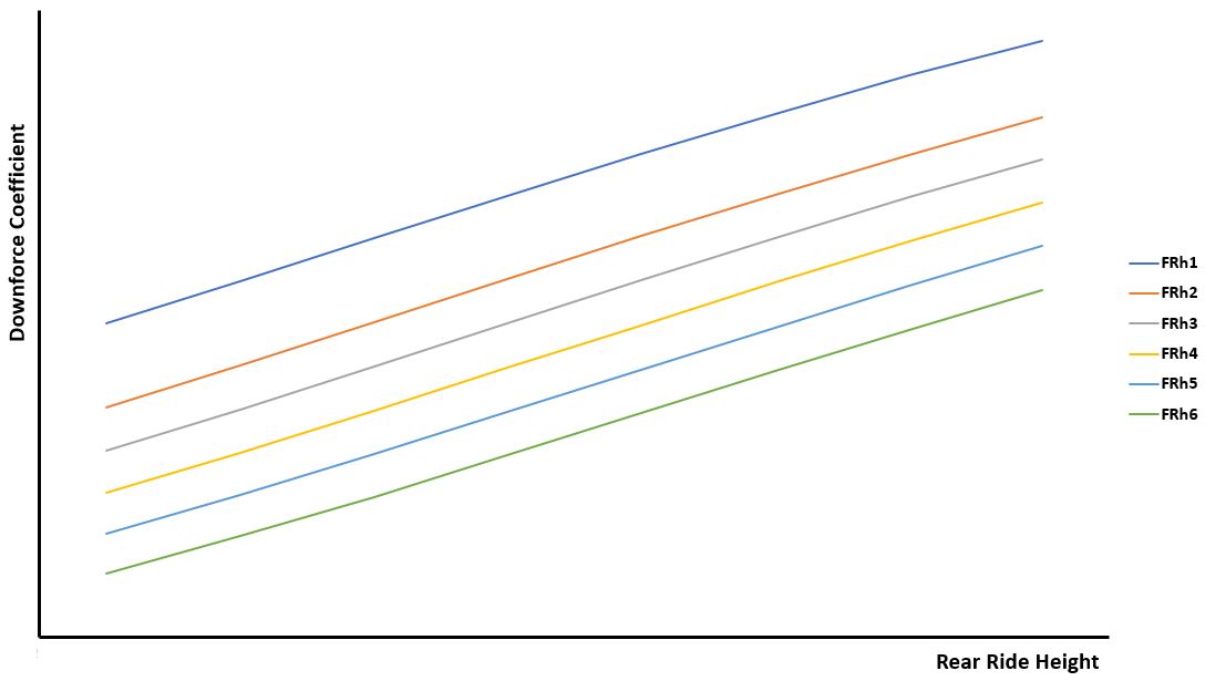
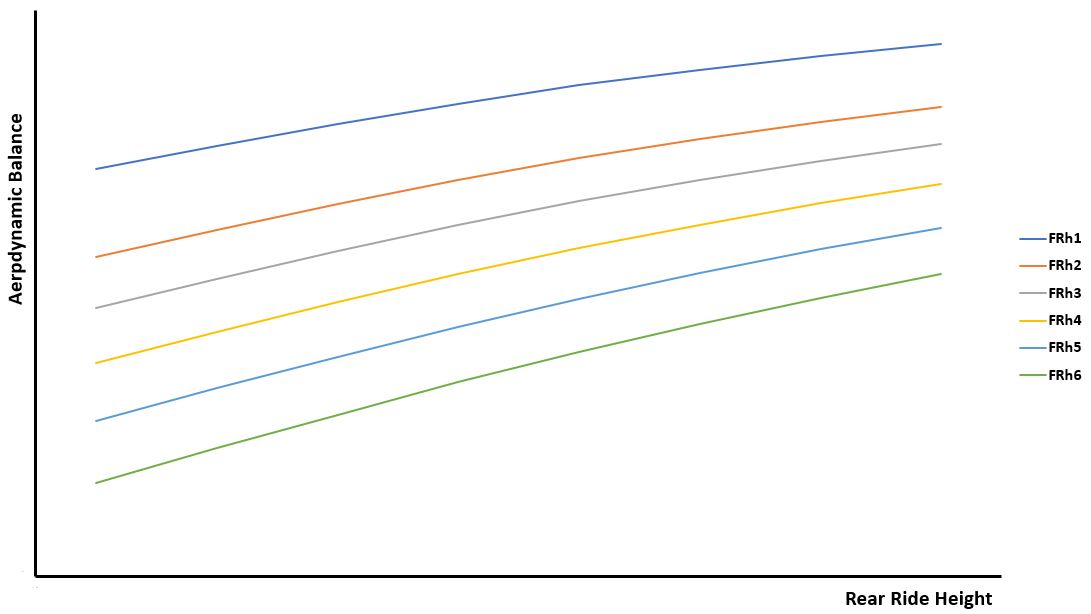
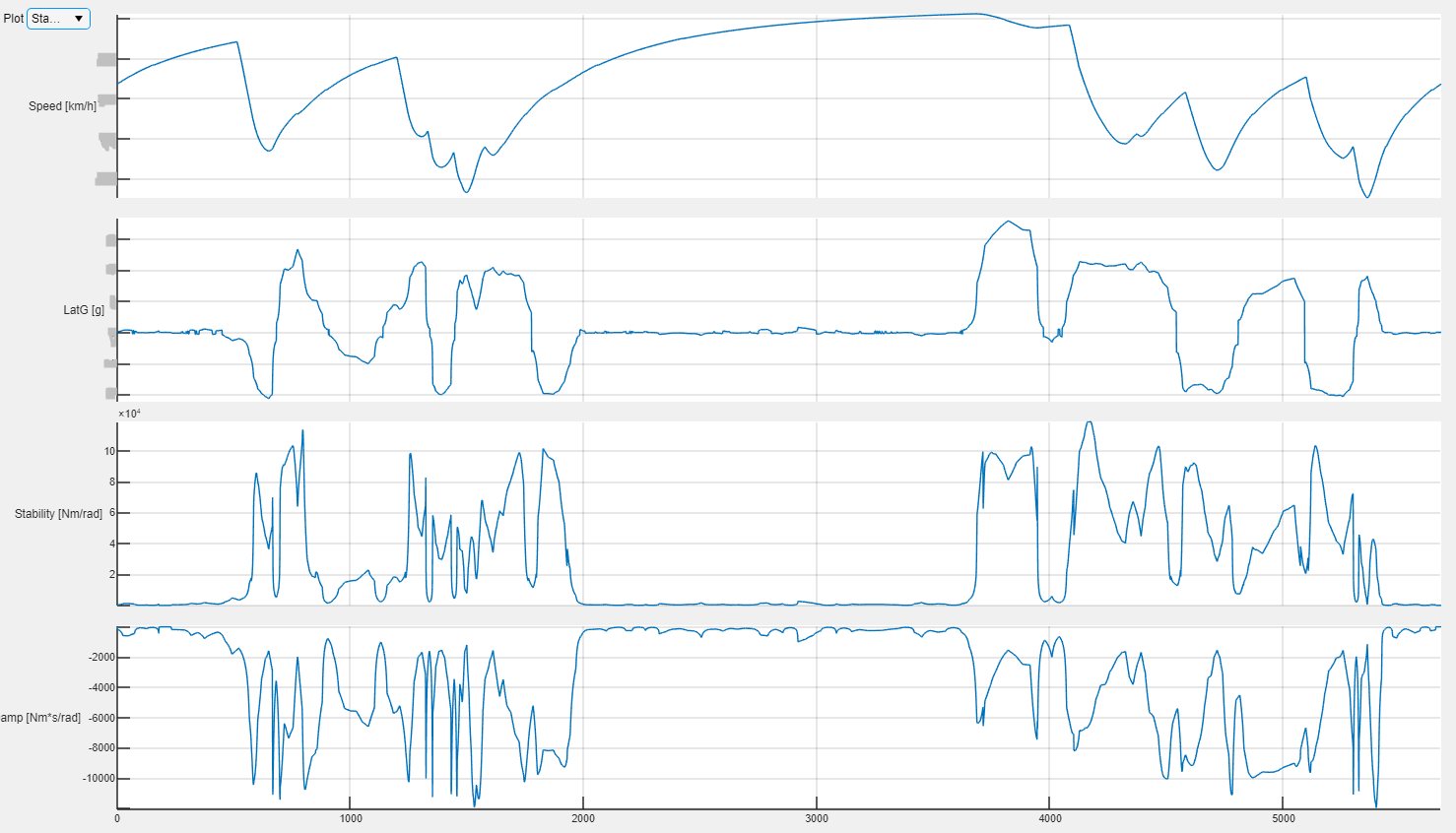
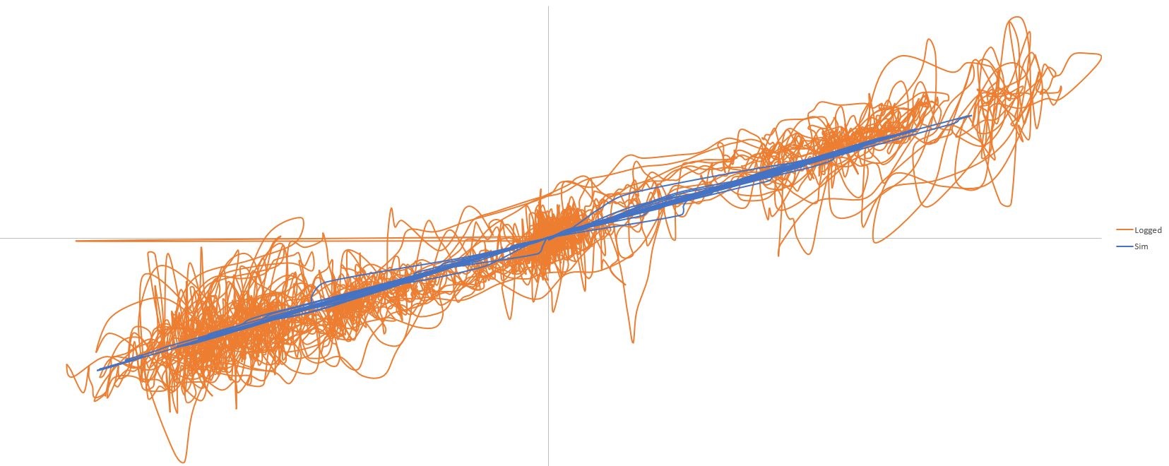
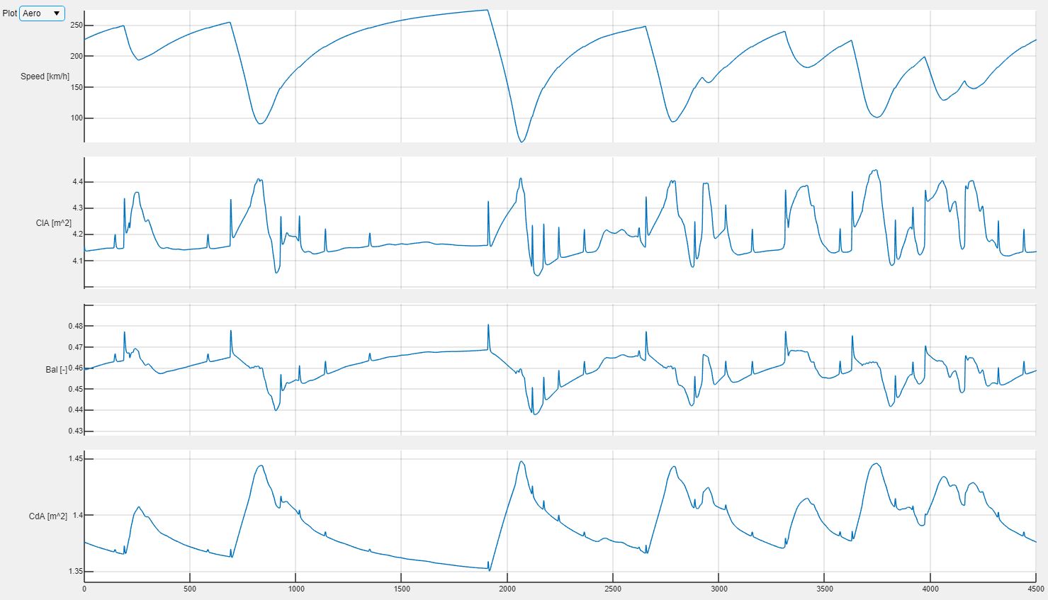
Linked to suspension travel, is how the aerodynamics performance of the car evolves during a lap, because of ride heights influence on downforce, drag and aerodynamic balance. The aggressive use of anti-effects described above has the main goal of controlling the aerodynamic platform, to maximize downforce and minimize center-of-pressure shifts.
Figure 5 helps to understand the effectiveness of the above strategy of using jacking forces to compensate third springs’ absence. Again, the first trace from above is car’s speed, followed by the downforce coefficient (ClA), the aerodynamic balance and the drag coefficient (CdA).
The aerodynamic balance trace has a spike only at the very beginning of braking phases, but this is relatively limited in magnitude. Despite the strong anti-dive limiting suspension travel, under longitudinal weight transfer the front wheels also deflects, producing a drop of front ride height and changing aerodynamic properties.
Immediately after, thanks also to the rear suspension going into jounce at the start of braking phases, the aerodynamic balance moves toward the rear and this should improve corner entry stability. This is particularly crucial in high speed corners like Turn 1 or Turn 9.
Another interesting element, also linked to suspensions heave stiffness, is how the drag drops at higher speed, something very beneficial for top speed. This is mainly due to pretty high rear wheel travels, consequence of relatively low rear wheel rates.
A similar high speed drop can be spotted on downforce too. Anyway, with respect to this metric, what is really interesting is how the downforce coefficient goes up again at the entry and at the apex of each corner, mainly due to the raise of rear ride height; once again, this is particularly important in high speed bends like Turn 1 and Turn 9.

First simulation results. From above: speed, downforce coefficient, aerodynamic balance and drag coefficient.

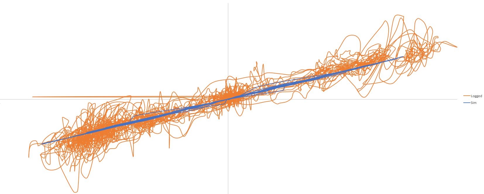
As discussed in my previous entry about Class One DTM cars, teams used pretty high static camber angles, as this seemed very effective in terms of performance and tyre exploitation.
Keeping in mind that the simulations described here do not consider any compliance, which would further push the outer wheels toward positive camber and the inner wheels toward negative camber (affecting grip negatively on both sides), it is interesting to analyze how each corner camber angle changes during a lap, under the effects of heave, roll and steering angle at the front. This is shown in figure 6.

First simulation results. From above: speed, front left camber, front right camber, rear left camber and rear right camber angle.

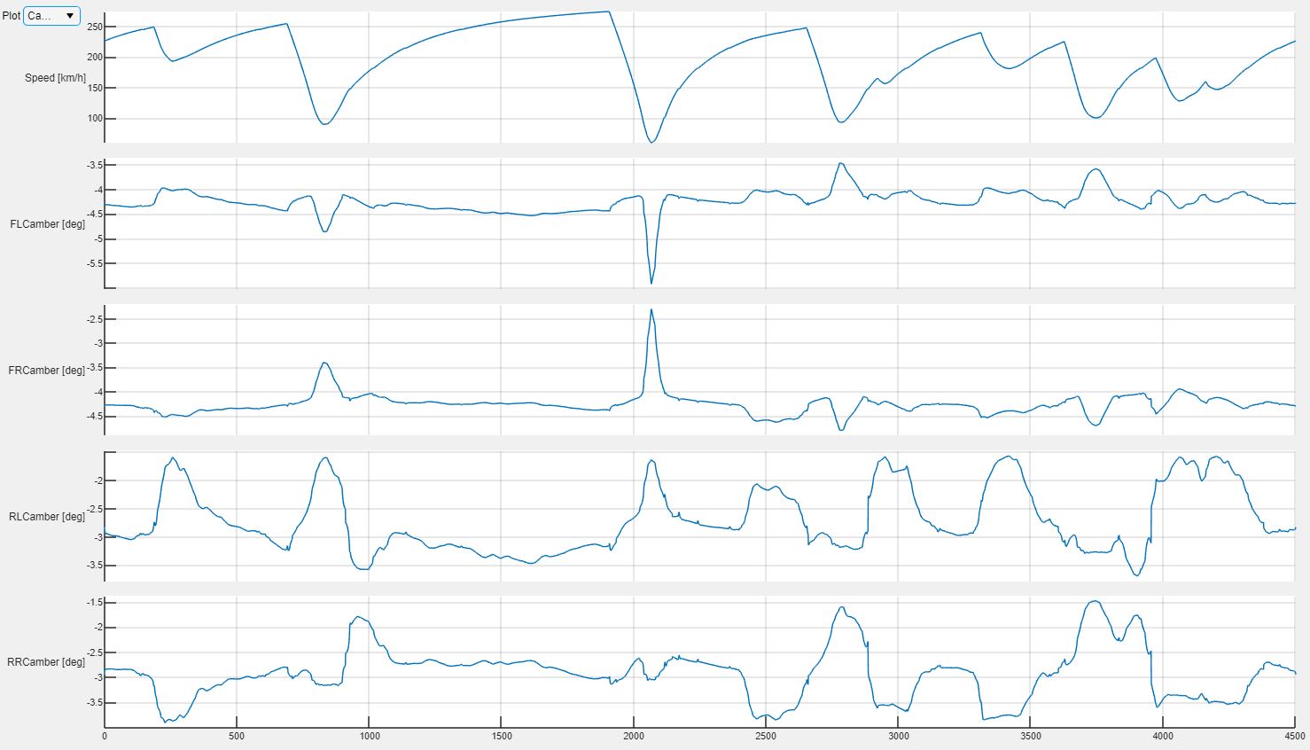
Focusing on the front axle first, we can recognize how, in slow corners, front suspension geometry, in particular with regards to caster angle, produces a significant camber change as a function of steering angle: for example in Turn 5, the front outer wheel moves toward more negative camber angles, presumably improving front axle grip and reducing understeer (typically an issue in tight corners). This happens mainly at the apex, where the steering angle reaches its peak. In corner entry, where the cars starts to roll but the front wheels are not yet steered much, the outer wheel experience initial positive camber change, instead.
On the other hand, in fast corners like turn 1, front outer camber goes toward positive values, compared to the previous straights, because roll stronger effect compared to the low steering angle required in higher radius bends.
On the rear axle, instead, in each corner roll pushes the outer wheel camber angle toward more positive values and, most probably, in a window where lateral grip drops, thus making camber gain with wheel travel even more important.

Sensitivities
How sensible is the model to a change of some of its main features?
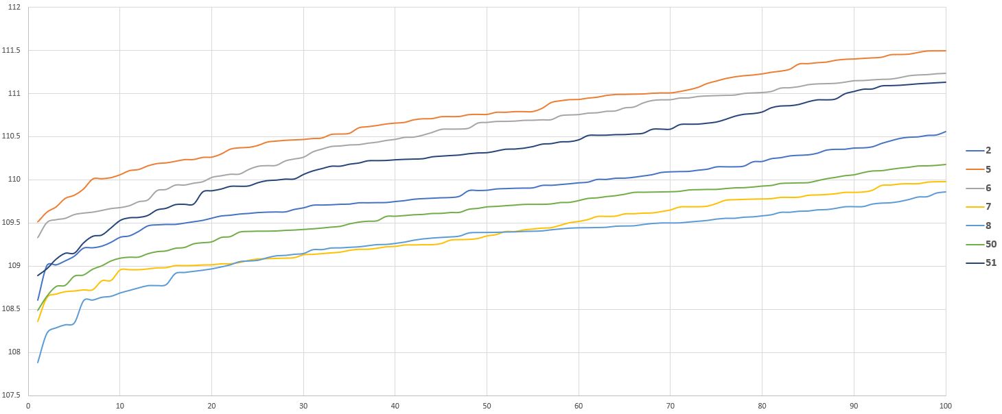
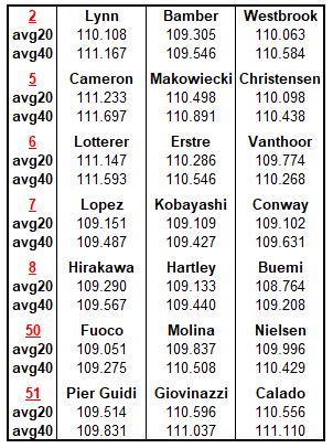
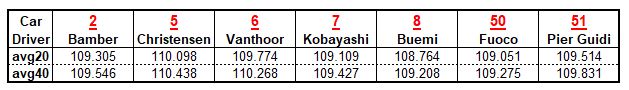
The results obtained varying some key parameters are summarized in the table in figure 7 . Here, each sector time (identified as S1, S2 and S3), the final lap time (LT), top speed (TS) and the differences (both in absolute and relative terms) to the baseline are provided.
All these runs have been performed without activating the DRS.

Basic lap time sensitivity to some key parameters

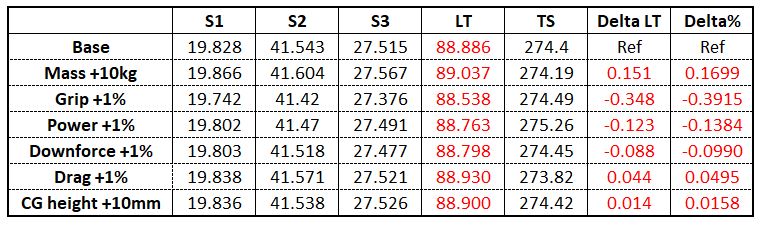
Keeping in mind the uncertainty relative to the tyre model, it is clear how grip is surely the stronger performance driver; this is actually no surprise, above all in a track where the car negotiates most of the corners in grip limited conditions.
Mass is the second strongest performance driver. In a class with a mandated minimum weight, one could think mass would not be an important parameter. Anyway, a too conservative approach with respect to the fuel load would change the overall weight, for example. The above results show how each single kilogram of fuel would produce a sensible drop in performance and how important crews precise fuel consumption calculations were.
Engine power has, on this track, a stronger effect on performance than downforce. It is also no surprise, that increasing engine power leads to an improvement mainly in sector 2, where the longest full throttle section of the car is located.
In terms of aerodynamic, having more downforce seems more effective than trying to reduce drag.
The CG height has a very small effect on lap times, instead.

Tyre management
As discussed already, an extremely important topic for last generation DTM Class One cars was tyre degradation.
The simulations we are analyzing refers to qualifying conditions, while tyre degradation is a topic mainly related to races. Still, it is possible to analyze how certain parameters influence not only final performance, but also the stress that the tyres experience on track.
To do this, we will look at tyres friction energies. They do not tell the complete story about tyres stress, but are relatively easy to calculate, give a decent picture about what happens to tyres outer layers and are a reasonable way to quantify how a certain set of parameters changes the way tyres are exploited with respect to a given reference.
As mentioned, teams used a relatively front biased weight distribution and tried to avoid moving mass towards the rear of the car to try and relieve the rear tyres a bit. It this also effective in terms of lap times.
The table in figure 8 considers the baseline run and two further ones, where the static weight distribution was moved respectively 1% toward the front and toward the rear.
It contains again sector times, final lap time, top speed, lap time variation in each run and each tyre friction energy delta, compared to the baseline. 

Effects of changing mass distribution on lap times and tyre friction energies

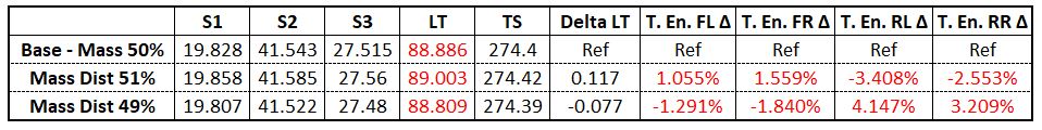
A more rear biased mass distribution produces better lap times in simulation environment with the considered tyre model. We could acually ask ourselves if the same would be true on a real track with a real driver: simulation models are most of the times front grip limited in cornering conditions (understeer), hence any setup solution helping to exploit the rear tyres to a bigger extent would help improving cornering speeds. This normally also produces a more oversteery car though. Would our DTM drivers like this? A higher rear axle saturation generally means a lower stability. This could be effective in qualifying, for a flying lap, but could be detrimental for driver’s confidence during the race, where tryre degradation would further move vehicles balance toward oversteer.
What is clear is that lap times improvements linked to a more rear biased mass distribution are achieved anyway at a price of a bigger friction energy (and, hence, degradation) for the rear tyres.
Shifting mass distribution 1% toward the front produces a bigger lap time delta than doing the same toward the rear while rear tyres energies are always more affected than front tyres ones from any shift in mass distribution.
Moving mass toward the rear normally also improves traction out of slow corners, beside the effects described above. This means both bigger rear lateral forces and longitudinal forces: both factors increase the stress experienced by the rear tyres.

DRS optimization
We will now focus on an example of how teams could optimize DRS deployment, to get the maximum lap time gain.
I could identify five zones, where the DRS can be activated complying to the rules:

1. Turn 1 – Turn 2
2. Turn 4 – Turn 5
3. Turn 5 – Turn 6
4. Turn 8 – Turn 9
5. Turn 14 – Turn 1

Another possible application zone would have been between turn 6 and turn 7, but that section is very short and I neglected it.
The lap time gain obtained activating the DRS in each zone depends not only on the assumptions considered in terms of drag, but also on the effective distance over which the DRS remains open. The simulation runs produced the results summarized in figure 9 table.

Lap time improvement with DRS activation

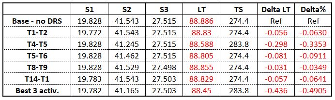
As we could expect, the biggest gain is produced between turn 4 and turn 5. This is not only the longest activation zone, but also the section of the track where the highest speed is achieved.
The best three zones identified in the table in figure 9 are indeed the longest sections of the circuit where DRS can be deployed.
Ideally, one would want to activate the DRS from the exit of turn 5 to turn 7, but even if, in normal circumstances, in turn 6 the car does not operates in grip limited conditions, the lateral acceleration overcomes the threshold mandated by the rules for DRS activation. Moreover, the rear downforce reduction and consequent forward aerodynamic balance shift would make the car pretty unstable.
The total lap time drop thanks to DRS is 0.436 seconds and the final simulated lap time is 1’28.450, that is reasonably close to 2020 pole position (1’28.405 for race 1 and 1’28.337 for race 2), taking also into account that these simulations did not consider the P2P.
Also in 2019, when the rules did not allow any DRS deployment in qualifying, the pole position time was a 1’28.972, that is not far from the 1’28.886 this vehicle model produced without DRS.
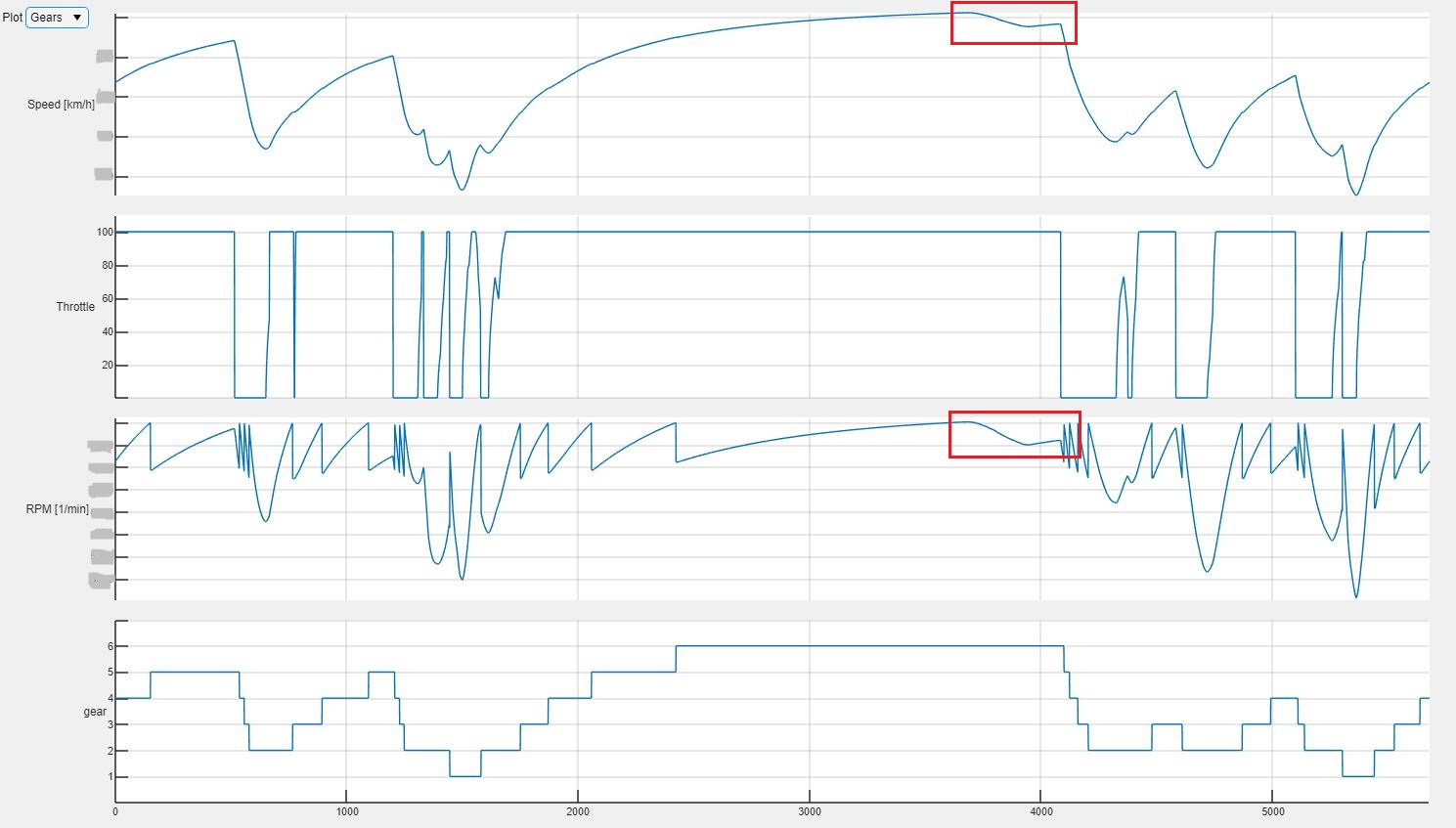
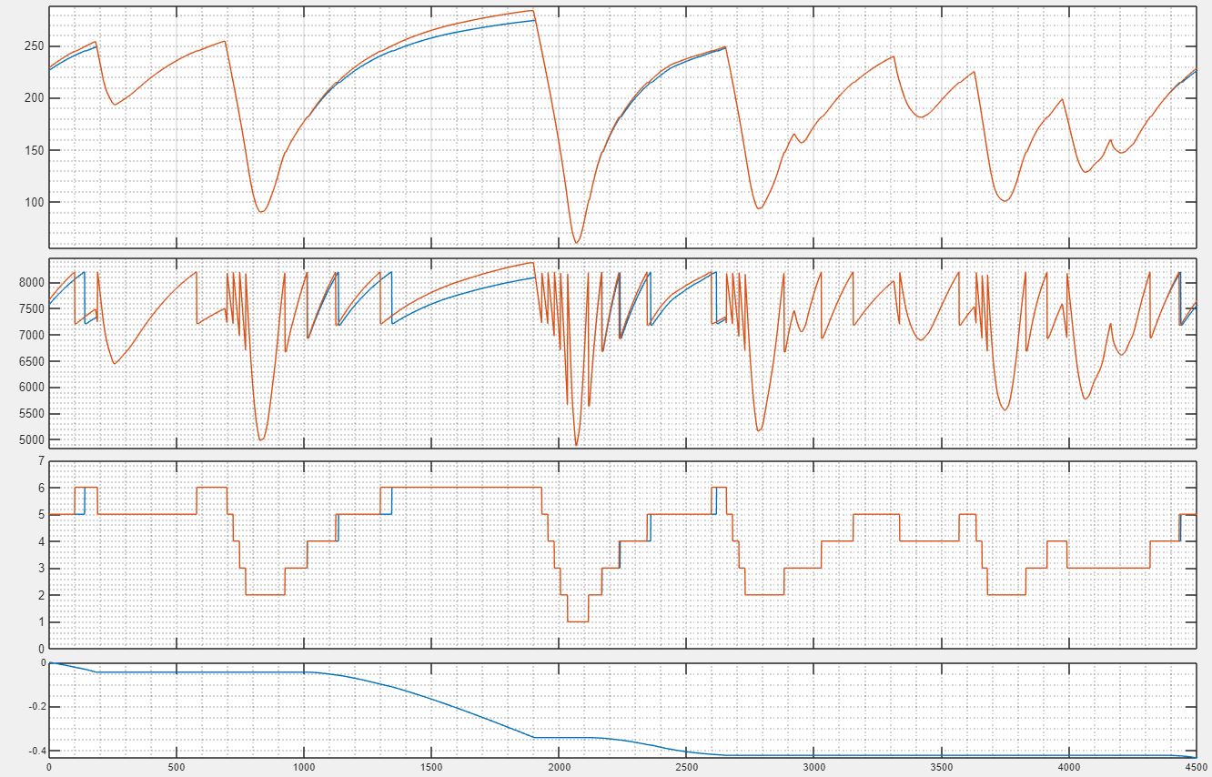
Figure 10 offers a comparison between the baseline run (in blue) and one with the DRS open in the three best zones (in orange).
Shown traces from above to bottom are vehicle speed, RPM, engaged gear and the compare time between the two runs.

Simulation results without DRS (blue) and with DRS activated in the three best zones (orange). From above: speed, RPM, engaged gear and compare time.

This closes the series of three articles where i tried to present a deeper dive into the latest iteration of Class One DTM; the aim was to better understand both the regulations and how the teams explored them to extract the amazing performance these cars produced on track, despite all the imposed limitations. For me, this was another extremely interesting application of lap time simulation, even with a simple tool like mine; this still allowed to analyze into details the effects of both design and setup parameters both from a performance and handling perspective, helping understsand not only how fast these vehicles were but also why.

Hi everybody,

this entry is the second part of a series of three articles about the DTM Class One cars.

Last time I provided my take about some of the main points of last generation Class One regulations and tried to highlight the main differences compared to previous, pre-2019 iterations and focusing on some of the areas that aimed at controlling performance and cost. I tried to focus on some of the elements that determined why the Class One ruleset was still able to produce incredibly fast cars and stimulate engineers so much, despite all the imposed limitations.
Today I will dive deeper into each area of the car and how far the team went trying to optimize every detail, while facing the challenges posed by the rules.
This analysis will form the basis on which a representative simulation model of a 2020 DTM car will be built and used for simulation purposes (next and last entry about this topic).

Regulations, aerodynamics and tyres
As every modern, high downforce racecar, aerodynamics was a very critical area for Class One vehicles in terms of performance and they were extremely sensitive to how ride heights changed dynamically. It is no surprise that teams focused very carefully on ride heights control on track.
To put things into context, a 2020 DTM vehicle, with the DRS deactivated, had possibly a higher downforce than a current Le Mans Hypercar, as an average on the aeromap covering the same ride heights range. DTM cars were developed to work in a bigger range of ride heights, though, above all at the rear, where suspension vertical stiffness was significantly lower than what one could expect in a Le Mans Prototype. As discussed last time, anyway, Class One cars had a lower aerodynamic efficiency, mainly because of their drag. To put this again into context, the information I collected suggest that their drag was probably more than 30% worse than that of a current Le Mans Hypercar.
The data I could put my hands on suggest a pretty linear relationship between downforce and rake; in other terms, for a given front ride height, downforce increases pretty linearly with rear ride height, without showing a proper maximum in the window the cars experienced on track. This seems to suggest that Audi’s intuition about a high rake setup was right.
The aerodynamic balance is also constantly increasing with respect to rake angle, but in a less linear way. Still, this seems to confirm how, in the range of ride heights the car worked in medium-to-high speed corners (where downforce plays a bigger role on performance) as well as during braking phases, the car could be effectively rebalanced using rear ride heights.
Lastly, as usually happens, drag had instead a much weaker dependence on both front and rear ride heights.

Downforce vs front and rear ride heights

Aerodynamic balance vs front and rear ride heights

The rules allowed only minor modifications on the cars after qualifying, while the big part of the setup had to stay the same for the race. Among the allowed adjustments between the two sessions, teams could work on brakes blanking. This is an interesting setup parameter because it influenced both brakes cooling and the aerodynamics of the car. Engineers used to adjust this not only to ensure the correct functioning of the brakes during the race, but also to influence the behavior of their cars. This tells much not only about how sensible the aerodynamics of these cars was, but also about the skills and sensibility of the drivers involved.
The rear wing angle could also be modified after qualifying, but its setting was often left untouched because mainly related to the overall drag and downforce level required by each track; blanking provided the engineers a fine tuning tool that could be used to adjust cars’ behavior more precisely.

Between qualifying and race, teams were also allowed to work on tyres, for example adjusting pressures. In general, tyres degradation was a very critical factor under the new rules, also because of the higher engine power stressing the rear tyres more than with previous generation engines.
Keeping tyres key parameters, like temperatures and pressure into the right windows was crucial to ensure higher performance, but also to keep the balance of the car as stable as possible during the race, before the mandated pitstop.
A widespread approach to try and limit tyre degradation and its effects on car balance, was to intentionally build into the car as much understeer as the drivers could accept for qualifying; the rationale behind this is that car’s handling would move anyway towards oversteer during the race, due to the generally quicker degradation of the rear tyres and, as described, because no major setup change was allowed in between qualifying and race. A more understeering setup would naturally balance this tendency, avoiding the car becoming unstable at the end of a stint.
Finding detailed information about 2020 DTM tyres was extremely complex. Tyres data are, in general, as desired as difficult to find, in many classes in motorsport. What is clear is that the products Hankook developed for the DTM had a pretty high vertical stiffness and decent grip levels in qualifying, but a pretty low durability. Qualifying cornering performance were pretty good, but drivers had to manage the tyres carefully during races.
As a general approach, teams run pretty high camber, with static settings up to 4 degrees at the front and above 2.5 at the rear. This seems to suggest that either DTM Hankook tyres produced better grip with a bigger inclination angle or that the teams were pushed in this direction by other effects: a reason, for example, could have been the camber loss produced by suspension compliance: under external forces at the contact patch, the suspension assembly undergoes deflections, that could lead to a dynamic camber reduction compared to kinematics effects (like roll) alone.
In terms of kinematics effects, anyway, also the pretty high roll angles, consequences of cars’ relatively low roll stiffness could have been a driver for needing high static camber angles.
This was probably very likely above all at the rear, while at the front axle a positive contribution with respect to dynamic camber was surely delivered, at least in tighter corners, by the relatively big caster angles. The teams were reported to run up to 15 degrees of caster and this surely helped to fight understeer in slow turns, as caster can usually be associated to a pretty marked camber gain with respect to steering angle, beside reducing the load transfer experienced by the front axle.
Another interesting (despite not uncommon, in modern racecars) solution adopted by Class One cars was attaching the pushrods to the uprights, instead than to the lower suspension arm; on the front axle the location of pushrods pickup point on the upright could be changed in longitudinal direction and this offered a further setup option to counteract slow corners understeer, by tuning how much the inner wheel load would increase depending on steering lock.

Active approach
In general, because of the extremely high level of the series and the very small gaps in terms of lap times, teams and manufacturers tried to optimize every detail of their cars for every track, doing relatively important setup changes also during the same weekend. Some areas, in particular, were given special attention, because of the big influence they had on performance.
A critical setup parameter for a racecar is the longitudinal position of the center of mass of the car and DTM vehicles made no exception. Because of the front engine, Class One cars had a pretty even mass distribution, with the amount of weight acting on the front axle being in the region of 50% and with the possibility to change this a bit, thanks to ballast. Teams worked very actively on mass distribution by moving ballast in different, predefined locations; the ballast was attached either to the upper side of the underfloor, of the front splitter or of the rear diffuser and was even used to adjust corner weights. The cars were slightly underweight and teams could play with 10 to 20kg of ballast (depending also on driver’s weight) to adjust the weight distribution to their needs.
Beside ballast, the teams went so far in weighting each component and spare part of the car they had in the workshop and purposedly mounting the lighter or the heavier to further adjust the mass distribution, if required. Bodywork and, in general, parts built out of composite materials are a often a good example of components where the weight can change a bit.
Beside considerations related to pure performance, many teams tried simply to move the weight distribution as much towards the front as possible, to reduce rear tyres stress and try to reduce rear tyres degradation.

Because of the crucial role played by the aerodynamics on performance and the very high sensitivity of downforce and aerodynamic balance to ride heights, teams paid great attention in keeping the car in the right window in terms of platform attitude and distance from the ground. At the front, this basically meant running as low as possible, readjusting the static and dynamic rear ride heights depending on rear wing setting, to change the center of pressure position as desired or stopping it from moving too much in certain situations.
As discussed last time, not having third springs to play with nor usable bump stops, the teams went very aggressive in terms of anti-dive and anti-lift, to control the aerodynamic platform mainly during braking phases. Cars were set with different geometries (by changing the suspensions pickup points) from track to track and, sometimes, even during the same race weekend. Very often, teams went so far with this approach, that even under a strong deceleration, the cars would not really compress the front springs at all and, in the very initial phase of the braking maneuver (when the forces are higher), the rear suspension would even go initially into jounce (instead of rebound, as one would expect during a braking phase). In other terms, both anti-dive and anti-lift were set often to values well above 100%.
Anti-dive and anti-squat settings need to be considered in conjunction with front and rear suspensions vertical wheel rates, as all these parameters contributed to optimizing the aerodynamics and platform control. Wheel rates could change a bit depending on track characteristics (for example, to comply with more or less bumpy surfaces) but, in general, Class One cars used to run with a relatively high front vertical stiffness and a pretty low rear one. Racecar Engineering sources revealed that front wheel rates were in the region of 200 to 250 N/mm per corner, while the rear would stay below 100 N/mm. Audi, in particular, with their high rake approach, would use this parameters to further contain front wheel travels in braking, while profiting from bigger rear wheel travels: this would, for example, allow the car to squat significantly at the end of the straights, under aerodynamic load, reducing overall drag. Moreover, lower rear spring rates helped to be more gentle on the rear tyres, to keep their degradation under control.
Interestingly, geometric anti-roll effects (roll centers position), seemed to play a less important role and were apparently often subject to compromises, as focus was put mainly on ride heights control.
As for antiroll bars stiffness, some teams had a pretty low front roll stiffness and a significantly higher rear one. Typical front, single-wheel-bump rates in roll were about 50 N/mm, while the rear had about twice that much. This goes in the opposite direction to what teams did with respect to vertical stiffness and was probably meant to compensate also for that, by getting both the overall roll stiffness and lateral load transfer distribution to the desired values. In general, Class One cars roll stiffness was not particularly high.
Another interesting area the teams used to further adjust cars’ balance was the differential. The rules mandated the ramp angles and the overall number of friction plates that had to be use inside this component. Anyway, teams were free to set the order of the friction plates, as well as change the preload. Racecar Engineering understood that teams tended to work on this mainly to improve braking and corner entry stability, by running pretty high preload and locking effect in coast.

Powertrain, Push-to-Pass and DRS
Given the boundary conditions provided by the rules for the latest generation turbocharged engines, what did the manufacturers achieved with this units?
In general, as for road cars units, one big advantage of turbocharged powertrains is the potential of having a pretty flat torque curve, for a big part of the engine operating window. Sources confirmed that was the case for DTM engines in the lower 2000-2500 RPM of the actual on track used range, while the maximum power was achieved pretty early afterwards, with the power curve remaining pretty flat up to the shifting point. This ensured a very high drivability.
Some engines were reported to rev higher than others anyway, as briefly discussed last month, Audi seemed to have found an edge on the competition in this compartment.
The information I could get tell about a maximum power in the region of 610-615 hp. Teams optimized the shifting point depending on the engaged gear, to further improve straight line acceleration.
Because of the favorable torque and power curves characteristics, teams used to set up the drop gear (the only tunable parameter allowed for the gearbox) for each track, basing on the expected top speed with the DRS open. With this respect, the target was to achieve the maximum speed at higher revs than the shift point itself, which was already after the point where the engine produced its maximum power; this means, at the maximum, DRS driven top speed, power probably dopped already a bit; this enabled anyway to still have a slight advantage during acceleration phases.
In general, having a pretty flat power curve after the peak ensures a greater flexibility, in terms of usable window.

The edgy power curve used for the simulation model, basing on the information I got.

Despite all the limitations that have been described, DTM latest ruleset maintained the DRS (Drag Reduction System) and the P2P (Push-to-pass); they were mainly meant to ease overtaking maneuvers during races, but also made the cars faster over a lap and became a performance boost in qualifying in 2020, when the teams have been allowed to use them also during these sessions.
The DRS worked analogously to the system that Formula 1 employs already since many years; its functioning was fairly simple: the system reduced the angle of the big, single element rear wing, thus reducing drag and increasing top speed. The maximum allowed angle reduction was provided by the rules (18 degrees) but, while remaining below this upper limit, teams could adjust freely rear wing incidence.
The P2P, on the other side, allowed the engine to operate for a limited time (5 seconds) at an higher fuel flow rate (100 kg/h instead of the normal 90kg/h), thus boosting its power by about 30hp, according to what the manufacturers reported in the press.
The DRS could be activated three times per lap, the push to pass only once. During the race, the teams had a maximum number of activations for the P2P.
These two elements provided the teams some low hanging fruits that could be used in qualifying to improve the ultimate performance of the cars over a single lap. In other words, these devices could be seen as an “easy” way to improve lap times, without investing huge resources in development. Anyway, also for the DRS and P2P, each manufacturer needed to analyze each track characteristics and identify where their usage would provide the biggest advantage, while complying with the restrictions given by the rules, that did not allow, for example, to activate the DRS in certain situations, as described last month.
While it is difficult to quantify exactly the performance gain produced by the P2P, as its activation was limited in time, DRS effects could be isolated in an easier way. My sources indicated how, in Hockenheim, the DRS would mean a top speed increase of about 9 kph; according to author’s results, this should mean a drag drop between 15 and 20%, compared to cars’ high downforce configuration of the rear wing.
Beside the positive effect on top speed, anyway, the activation of the DRS also meant a significant drop of rear downforce and, as a consequence, a sensible shift of the aerodynamic balance towards the front. This is something that could be clearly seen analyzing logged data, in the form of a strong reduction of rear suspension travel, immediately after the DRS was engaged. Among the consequences of such a sensible center of pressure shift towards the front, there are of course a strong reduction of vehicle’s stability, but also an increment of rear tyres slip, that could lead to a faster temperature increase than in normal conditions.

Vehicle model
As I mentioned, while finding the information described above has not been easy, because of the high secrecy surrounding Class One cars (as happens in every championship where mainly works teams take part), this has allowed to build a pretty detailed vehicle model, that could be used to run different kind of simulations and analysis.
These should provide a better picture not only of the performance of these cars and how this was achieved, but also lap times and handling sensitivity to some key design and setup parameters.
All of this will be the subject of the next entry about DTM Class One Cars.

Hi guys,

this entry will be a bit of a “back to the future” moment, as I will try to analyse the first 2023 WEC Race in Sebring, basing on the publicly available data and focusing only on the top class.
It’s a long time since analyzed a race here, but the new era that started in Sebring for the Hypercar class, with the convergence of LMH and LMDh regulations and seven different manufacturers competing against each other in the top class has provided enough motivation to try and look into the numbers.

The class is surely one to watch, with the like of Toyota, Ferrari, Peugeot, Cadillac and Porsche fighting each other for victory. Particularly interesting, the cars taking part respond to slightly different rulesets.
LMDh vehicles comply to IMSA regulations and are based on chassis provided by four manufacturers (Dallara, Oreca, Ligier and Multimatic) that OEMs can use to attach their own powertrain and create styling cues of their production cars. Those chassis will also for the based for the still-to-be-born future LMP2 class.
These cars are RWD only and have an hybrid powertrain where the electric system (producing a maximum of about 50 kW) being a spec part and is produced by Bosch.
LMH cars, on the other hand, are developed from scratch by each competitor; they are free to design and build each small component of their car as the please, as long as they respect the ruels, and can (but must not) use an hybrid system on the front axle, thus making the cars “part time AWD”. The front electric motor can produce a maximum of 200 kW. To balance LMH cars more fairly against LMDh vehicles, the electric motor can transmit torque to the front wheels only above 190 kph, with the only exception for Peugeot (also because of their tyres, see later) that can profit from a AWD powertrain above 150 kph.
Non hybrid cars can be employed too: in that case, the powertrain can only drive the rear wheels.
To balance the two different concepts and keep the performance of the cars in a given window, the rules needed to be pretty complex, as one could expect, despite said performance being actually significantly lower than what the old LMP1 cars could produce.
The power at the wheels at any time must be below a given curve, that is provided by the rules and can be adjusted up or down, and with the maximum power moving between 480 kW and 520 kW (maximum reference power 500 kW).
The aerodynamics of the cars is also tighly regulated and downforce and drag must be inside specific windows, defined basing on the drag in end-of-straight like conditions and an weighted average of the downforce map.
The tyres are produce by Michelin and are the same for everybody. All cars except Peugeot use 29/71-R18 front tires and 34-71/R18 reear tires, while the French team was allowed to employ 31/71-R18 tires all around, because from the beginning the developed their car around a choice and a late change would have been too complex.
Minimum weight must be above 1130 kg without driver and fuel, but many of both LMH and LMDh cars have been given a higher minimum weight for the first races of the season.

Despite being much slower and (hopefully) cheaper and less technologically complex than the old LMP1 beasts, the hypercars have surely still caused some headaches to the engineers working on them, because the rules still leave enough room for “optimization”. Looking at the aerodynamics, for example, as the performance are tighly regulated, some teams underlined how their effort was focused on producing a car with a big driveable window as possible.
Beside this, as the downforce is regulated in the form of an average over the aeromap, one could think efforts have also been spent on exploting the regulations in the best possible way, maybe by having region of the map where the DF is higher, accepting to be penalyzed in other regions to counteract.

Sebring
The race was won by Toyota, who produced a 1-2 in dominant fashion. Ferrari had suprised the field by taking the pole position in qualifying, but had both less pace and some mistakes compromising any chance of victory during the race. They italian team still finished third at their debut on a very special and demanding track.

Sebring is indeed a special place, extremely bumpy, with a mix of asphalt and concrete surfaces and a combination of low, medium and high speed corners. The 6019 meters long track was divided as usual in three sectors, as shown below.

Sector 1 is opened by turn 1, the fastest corner of the track, but is also dominated by Turn 3 and 5, with the latter being pretty important for lap times, because it leads to a fast section of the circuit.
The corners having a stronger influence on lap times are anyway slow-to-medium speed ones, in particular T7 in sector 2 and T17 in sector 3, with the latter being probably the most important in terms of final performance.
The first sector is the only one including a proper fast bend, still each sector has a combination of very different corners in terms of minimum speed, making downforce still a dominant factor for performance.

Because of Sebring very specific charachteristics, it is reasonable to think that teams who collected more experience in this circuit, either because they raced here in previous seasons (see Toyota) or because they tested before the race, could have a substantial advantage. With this respect, even if seeing a manufacturer struggling so much was surely strange, one could imagine that Peugeot was at disadvantage compared to Toyota, but also against Ferrari (who tested in Sebring before the race) and teams racing LMDh cars, like Cadillac that also race in the IMSA Weather Tech Championship and had done so with their previous DPi machine from 2017 to 2022.


BoP
Very important in terms of performance was of course also the BoP used for this first race of the season. The renewed system will not apply BoP changes on a race basis, but those will stay constant for a longer time. After Sebring (where specific values were applied), the BoP should not get changed for the following three races, that also include Le Mans.

In Sebring, the maximum power and minimum weight for each car were as follows:

Toyota: 1062 kg, 517 kW
Ferrari: 1057 kg, 515 kW
Peugeot: 1049 kg, 518 kW
Porsche: 1048 kg, 517 kW
Cadillac: 1038 kg, 513 kW
Glickenhaus: 1030 kg, 520kW
Vanwall: 1030 kg, 511 kW

It was of course not nice to see how LMH class privateers (Glickenhaus and Vanwall) struggled in Sebring.
While Vanwall was new to the class, the American team actually raced here already and with decent pace too. In all honesty, I think few had expected the privateers to have the same pace as the big manufacturers: Vanwall seemed to struggle with reliability and this is probably normal with a new car. But it would be interesting to see how Glickenhaus will perform in the next events in Europe, before Le Mans, as they did not surprise in a positive way in Sebring; many were expecting Glickehnaus to perform better (they had the best BoP of the class, staying at the minimum weight and maximum power allowed by the regulations) and have better reliability.

Performance Analysis
Now to the interesting numbers.
As already mentioned, Toyota dominated the race, with an amazing pace and a perfect execution. Their two cars had similar pace and probably also managed fuel consumption very intelligently: both crews could be heard lifting and coasting before braking points already during the first laps of the race and, realistically, until the end. The winning car could even avoid a final pit stop by saving fuel in previous phases. This is reflected by the data. Let’s take a look.

Average of the best 20, 50 and 100 lap times of some of the LMH/LMDh cars

Beside confirming that Toyota had a sensible advantage on the rest of the field in terms of pace, the above tables underline how the closer crew in terms of pace was Ferrari n.50, while the other italian car struggled more and felt also behind the Cadillac n.2.
Both Porsche cars were significantly slower than the Cadillac, despite belonging to the same set of tech rules. They apparently struggled with rear tyre degradations, already in the first hours of the race.
Peugeot was very far not only from the best, but also from the next fastest team. The French team was reported having severe issues in controlling their ride heights, partly also because they were probably not prepared enough to tackle the challenges of this special circuit.

The two Toyota were pretty close to each other. Anyway, it is interesting to notice how actually the winning car was slightly slower than Toyota n.8. The latter did a pit stop more than the sister car, when the Hartley drove into the pit twice in two laps, once under full course yellow and the second time immediately after the restart. The rules in fact did not allow to full refuel the car under full course yellow, as far as I got but the car needed some fuel to at least go on before properly refueling. Result was car n.8 spent about 41 seconds more into the pitlane than car n.7.
Car n.8 was also constantly and sensibly slower in terms of top speed than the sister car. While this could be down to a different aerodynamic setup, the difference could also be due to a more aggressive lift and coasting, at least when passing over the speed trap before T17 and this seems the most realistic scenario to me.

One final point to notice is how the Ferrari n.50 was actually closer to the two Toyota in sector 3, than in sector 1 and 2, thanks maybe also to an higher top speed. This could be related to a less aggressive fuel saving too.

All of this is graphically reflected in the picture below, depicting the best 100 laps of each crew. Lap time is on the vertical axis, while the horizontal one counts the laps.

Best 100 lap times of each of the considered crews.

The above plots do not consider the two Peugeot and the privateers, as they were sensibly slower than the rest of the pack anyway.

The lines relative to the two Toyota intersect two times, confirming how close the two cars were to each other. By looking a bit at the onboards and at the pit stops sequence, it looks like both cars were saving fuel but it could be realistic to think that car n.7 did this more aggressively towards the end of the race.
Ferrari n.50 was clearly the best of the rest. The sister car struggled much more instead and was sensibly slower than the Cadillac. One of the reasons for this difference, seems to be that car n.51 drivers are averagely a bit heavier than those wheeling car n.50.
Anyway, we will see in a minute how there are also other clear reasons for this difference.

What about each sector performance?

Beside the above table, how each car performed in each sector is shown clearly by the pictures below.

Best 100 sector 1 times for each of the considered crews

Best 100 sector 2 times for each of the considered crews

Best 100 sector 3 times for each of the considered crews

Toyota n.8 had a small, but consistent edge on the sister car in both sector 1 and 2. Considering everything, we are really talking about small differences here and it is really astonishing to see how close the two crews were to each other, in terms of performance. Still, a small advantage over an 8 hours race can make a difference and one could wonder what could happen without that double refueling for car n.8.
All the other cars, with the Ferrari n.50 on top, were left behind in each sector, but they surely struggled the most in sector 1 compared to the Japanese squad.
While Ferrari n.50 seemed to stay close to the Toyota if we look the best 20-30 sector 1 times, they fell behind on the long run (we will dig deeper into this later).
The Cadillac, the second “best of the rest” car, was, in relative terms, not particularly close to Ferrari n.50 in this section of the track, but surely better than all the others, Ferrari n.51 included.
As for Porsche, it is interesting to see how car n.6 was consistently faster than car n.5 in sector 1 and sector 2, with the difference in the first sector being pretty big. Aynway, the two cars were pretty close to each other in sector 3. A possible reason for this will become clear in a minute.

Sector 2 was a bit more favourable to car n.50, who kept a gap of about 0.1 seconds pretty consistently from the Toyota, above all considering more laps.
The Caddy was a bit slower than Ferrari n.50, but still better than car n.51, with Porsche being the slowest of the manufacturers again.

Both Ferrari n.50 and Cadillac were surely closer to Toyota (and to each other) in sector 3. Car n.50 in particular seemed to be able to keep both Toyota honest if we look to the first 20-30 best sector times, but felt behind when considering more laps. This is a point you should remember, as we will come back to this shortly.
Also the Cadillac stayed close to the top in sector 3. This could confirm that the two Toyota were managing fuel, as their top speed was also on the lower side of the pack, particularly considering car n.8 (see picture below).
Another interesting point, also related to top speed and fuel saving, is how in sector 3 the Toyota n.8 did not have the advantage they had on the sister car in the other sectors. This, together with the lower top speed, could maybe suggest how the crews were both saving fuel, but in different ways, with car n.8 maybe doing this more aggressively before the braking into turn 17, while car n.7 maybe was “distributing the effort” more evenly during the full lap. Of course, I have no specific data at my disposal to prove this wrong or true.

Interesting also to compare again the two Porsche. Car n.6 has a slightly lower top speed than car n.5. We have seen how sector 3 was the only one where the two cars had a similar performance, while over the rest of the track car n.6 was consistently faster. This difference in top speed could surely be one of the reasons, as a big portion of sector 3 is indeed the straight leading to turn 17, where also the speed trap is located.

Best 100 top speed marks for each of the considered crews

Was the advantage of the Toyota related only to their superior car?
Well, maybe not only.

The table below provides the best average 20 and 40 laps driven by each driver of each crew during the race.

Average of the best 20 and 40 lap times produced by each driver during the race

Before digging into any analysis, let me use a word of caution when looking at the above table. First of all, even assuming that each driver of each car left the pit at the beginning of each stint with the same amount of fuel as his team mates, I have no clue about the status of the tyres.
The tyres, in particular, seem to be an even more important topic than the were already. The new design brought by Michelin, which uses a more green approach and promise to be easier to recycle, and the ban of any kind of tyres warming device or procedure produced some troubles for the teams. Tyres are always very sensitive to track and ambient temperature, but it seems this was a bigger issue than ever in Sebring, as many struggled during the first laps with low grip and cold rubber.
Considering the race was about 8 hours long, it is no surprise that track and ambient conditions changed sensibly during the competition. Air temperature, for example, went from about 25 deg C at the beginning of the race, to about 29 more or less mid way, to less than 25 at the end. In the same time range, track temperature also changed from 32.5 deg C, to 42, to about 31 in the closing phases.
Beside this, I do not know if any car got any damage during the race, making it slower when a new driver jumped it.

After this premise, let’s look at the numbers, once again.
The first thing we can notice is that Toyota’s drivers were extremely well balanced in terms of lap times, with maybe the only exception of Buemi being slightly faster than the rest. All had very similar pace to each other and this could also be a testament to the car being easy for all of them to be driven fast in a consisten manner, and to the team doing a good job in managing the race.

This parity between all the drivers was absolutely not the case for the other teams.
If we look at Ferrari n.50, we see how Fuoco was much faster than his team mates, with an advantage between about 0.8 seconds and 1.2 seconds for the 20 and 40 best lap times average. This is a very big span!
The situtation was not much better for Ferrari n.51. Here, Pier Guidi was between 1 seconds and 1.3 seconds faster than his co-drivers (and this beside the n.51 car being constantly slower than car n.50, as we saw).
Also for Porsche, there was a pretty big difference between the fastest drivers of each car (Christensen and Vanthoor) and their team mates, with gaps spanning between 0.5 and 1.2 seconds.
The situation was only slighly better for Cadillac, with Bamber being clearly the fastest guy at the wheel.

I really need to stress this once again: these data need to be taken carefully, as we don’t know the conditions of track, car, tyres, traffic, etc. that each driver met during his stints. But I think they still show an important factor differentiating Toyota’s status to those of all the other teams, at least for now.

Without knowing how all of these factors played a role on each driver performance, we could wonder if the differences we see are down to pure driving, to the car suiting the driving style of certain drivers better or if some of the cars were simply harder to drive consistently.

Considering this latest comparison, what would the situation look like if we compared each crew to the others by only considering the best driver of each car? This is shown in the following table.

Comparison between the average of the best 20 and 40 laps produced by the best driver of each car

If we would assess teams performance only by looking at the table above, we would get a completely different picture.
First of all, Ferrari n.50 car would split the two Toyota, being slightly slower than car n.8, but also a bit faster than the winning car n.7.
Of course, one could ask what each car fuel strategy was. As discussed, it looked like Toyota was saving fuel during the race.
Still, we could say the Ferrari had pace, basing on this information only.

The other interesting bit is again the pretty good performance produced by the Cadillac, which was actually pretty close to both Toyota and Ferrari, above all if we look at the average of the best 40 lap times.

Of course, Sebring was only the first race and everything is new for every team considered in this analysis except Toyota. So it would be no surprise to see some serious progress for some of the competitors. This, or any BoP change, could surely provide some further excitment (or anger) for the fans!
The BoP will change slightly for the next races, until Le Mans, but hopefully coming to more traditional tracks, lile Portimao (that has been resurfaced in the last years and is not as bumpy as it was before) and Spa could produce some exciting show and closer racing.

Hi everybody,

and a very belated happy new year everyone.
Life comes always in the way of this blog, for some very good and some other less good reasons. The result does not change: I always wish I could write more and more often.

Since the year has just started (well, we had already the 24 Hours of Daytona and the debut of the new GTP class, actually) and I don’t have too much to share yet, I thought I would try something different today.
In fact, today and in the next future it will be about a series that has always fascinated me, from its start very long ago until what was for me its death, at the end of 2020. Part of this fascination came in the form of a child playing with RC cars made by Tamiya in the mid 90s.
The name of this series has always indicated this being a touring cars class, anyway very soon it became something very different and extremely exciting, from an engineering point of view.

A bit of history
I am not good in telling stories, and surely not in English, but I will try my best to avoid nonsense.
The Deutsche Tourenwagen Masters (before, Deutsche Tourenwagen Meisterschaft), in short DTM, has historically been one of the most competitive touring cars championships in the world and, in each of its eras, has always employed some of the most performant production-inspired racecars of the globe.
As its name suggest, this is a German based championship, whose generation can be dated back to the mid-eighties. Initially, the cars taking part where production based vehicles, tuned to be raced on track. Very soon, anyway, after works teams joined the class, the rules started to diverge from this principle, making the championship one of the most technological advanced classes already at the beginning of the nineties, when fierce battles between Mercedes, Opel and Alfa Romeo made up for a unique show.
The very open rule book though was the most appealing and, at the same time, the most dangerous trait of the class: a cost escalation lead to the championship cessation in 1996, after officially expanding also into the International Touring Car Series in 1995, a trophy made up of races all held outside Germany.

The series came to life again in 2000 and has since then always raced, while experiencing some significant regulation changes over the years. Despite the name, cars were at some stages actually based (in terms of visual cueing, at least) on 2 doors coupes, as in latest years. The high performance of DTM vehicles has always been a key point, anyway, despite the continuous effort of the regulators to reduce costs and slow the cars down, while trying to make races more entertaining.
With this respect, one of the key evolutions in terms of regulations was the introduction of devices and strategies to make overtaking maneuvers easier, like the DRS (Drag Reduction System), that reduces the rear wing angle and the Push-to-Pass (P2P), that ensures the engine some extra power for a limited time.
Moreover, since 2014 DTM and the Japanese SuperGT agreed on racing on the same base regulations, with the final move completed in 2019, when also the German series dismissed the naturally aspirated, gloriously sounding 4.0 liter V8 engines in favour of turbocharged, 2.0 liter units, similar to those already used in Japan. This new, international class, named Class One, offered the interesting prospect of having racecars based on the same rulebook and racing in national championships around the globe and, in some occasions, challenging each other in international events.
The DTM had constantly at least three manufacturers involved since the return of BMW to the series, in 2012. Anyway, at the end of 2018 Mercedes left the championship. In 2019, Aston Martin joined Audi and BMW but left at the end of that season already. Among other things, this lead Audi to leave at the end of 2020 too. As a consequence, the Class One regulations have been abandoned altogether by the DTM, in favour of a GT3 based set of rules that was implemented in 2021.

Since then, the series is still called DTM (recently the owner has even sold it to ADAC, if I got it right), but for me the DTM passed away in 2020.

Ok, I am done with the history review. Let’s come to more interesting stuff now.
This entry and the following ones about Class One will focus on the latest iteration of the technical regulations (2019-2020) and will be based on some pretty detailed data I could collect here and there and that allowed me to build a decent vehicle model and run several simulations with my lap time simulation tool.

This first article will serve as an introduction about what the latest iteration for the class was based on, from a technical perspective. The next one will be more interesting, with some numbers and plots. So I really hope my now 5 stable readers will not get too bored and read this and also the following posts.

Class One latest iteration
As I mentioned above, the latest iteration of Class One regulations was adopted in 2019, with the introduction of the new, turbocharged engines and some further changes aimed at reducing cars downforce and performance. The same year, the DTM and SuperGT held some common races where cars from both series competed against each other, both in Germany and Japan.
The baseline for the cars remained the same. DTM cars were meant to be front engine, rear wheel drive vehicles, with resemblance recalling manufacturers’ road cars. 
In 2020, some additional adjustments, mainly on the sportive side (for example enabling the deployment of DRS and Push-to-Pass during qualifying, previously allowed only during races) produced a drop of qualifying lap times, compared to 2019, but the technical rules remained the same.
In their latest form, the regulations implemented many limitations in different areas with three main goals: to slow the cars down, reduce costs and improve the show for the public. 
With respect to performance, the only factor going in the opposite direction was the engine, whose power went up significantly reaching peaks in excess of 600hp.
The general approach aimed at creating cars with more power, but less downforce and, hence, harder to handle in braking and corners. This, together with the availability of DRS and P2P, produced probably the most exiting races the series had seen in a long time, where both pure pace and strategy could be crucial for the final results. With this respect, an important role was also played by the tyres, whose high degradation forced teams and drivers into a careful race management; the rules mandated at least one pit stop.
Despite regulators’ efforts to control technological development, DTM cars maintained extremely high performances and the tight regulations pushed the teams into searching creative solutions in different areas. Since teams performance were very leveled, every little detail could make the difference.
In general, as a tech enthusiast, I am always puzzled when the regulators stop teams from using features that don’t really increase costs that much but make very much sense for an engineer (you will see what I mean very soon), but I must admit for this specific case, this probably made the engineering side of things even more interesting, up to a point.

The pillars of Class One regulations were, from a technical perspective, to impose the design, characteristics and dimensions of many performance critical areas of the car.
Manufacturers had to use many common components for their vehicles, the most noticeable one being the monocoque, surely the biggest single part of a racecar, with a crucial importance not only for safety, but also because every other major subsystem is attached to it.
Besides the tub, other significant examples were suspensions components, while the location of suspension pickup points had to fall into defined volumes, described in the rules as boxes of specified dimensions.

Suspension pickup points: example of allowed volume for suspension attachment location as mandated by the regulations

Key dimensions of the cars were also mandated; examples are the relatively short wheelbase (2750 mm), the maximum width (1950 mm) and, of course, the minimum weight, specified as the one of the car with the driver on board without fuel (1070 kg) .
Being such a critical area in terms of performance, aerodynamics made no exception to other compartments and the design of the lower part of the bodywork and the floor had to be the same for all cars, as well as the rear wing, rear diffuser and front splitter. Even if the general shape of the bodywork should have styling cues of each brand road cars, some areas of the upper part of the car also had to respect given positions or dimensions.
The powertrain area was also subject to tight rules. The engine itself, in line with what SuperGT employed already since some years, had to be a 2 liters, inline 4 cylinders unit and the fuel mass flow to the combustion chambers (direct injection) could not exceed 90 kg/hour.
The gearbox was another specified part and that included also the gear ratios, that were fixed, with the exception of the drop gears, that could be chosen among 11 allowed options, to adapt to different circuits requirements and to different engine characteristics.

Where did performance come from?
All these limitations surely had an impact on cars’ performance. The aerodynamic and engine power were surely responsible for the biggest effects, one in a positive and one in a negative way.
Interestingly, comparing qualifying lap times achieved in 2018 and in 2020 clearly shows how, in their latest season, DTM cars were faster than they were with previous regulations sets. Having a bigger engine power, as well as being allowed to use the DRS also during qualifying sessions were surely key factors.
Anyway, how much did the regulations really hurt or helped each area, performance wise and how did DTM cars build up performance over a lap?
In the past, finding any data about DTM cars was nearly impossible for anybody outside the official teams. Often, the team themselves did not have access to all the information relative to their own cars. Secrecy was a very high priority for the manufacturers.
Now that the Class One regulations have been dismissed, anyway, some people were a bit more open and provided some information. It was not easy to get enough to build a vehicle model and data came from very different sources. Some critical areas, like tyres, remained an unknown and I had to use data relative to other series using tyres of similar dimensions to approximate something, hopefully, realistic.
It was worth it, I think, as the lap time simulations I did help me to understand not only how these cars performed and handled, but also why and this was surely very intriguing.

Aerodynamics
As I mentioned, some of the strongest limitations in terms of aerodynamics, compared to previous years, were related to the front splitter and the rear wing.
Comparing 2019 cars to 2018 ones, one can clearly notice how the front splitter had to have smaller dimensions, while the rear wing had to be wider and composed by a single profile. This had to produce a downforce drop and make harder for the manufacturers to achieve the desired aerodynamic balance, further limiting cars overall performance. Moreover, the big, single element rear wing made the drag reduction, as a consequence of the activation of the DRS system, more sensible, thus ensuring a stronger effect in overtaking maneuvers, improving the spectacle for the public.

Differences between 2018 (below) and 2019 (above) DTM cars. The front splitter became much shorter in 2019.

Differences between 2018 (on the right) and 2019 (on the left) DTM cars. The rear wing switched to a single profile and got wider.

Some very nice aero guys explained to me how the biggest challenge was actually to ensure a proper cooling for the new, turbocharged power units, that were more demanding than the old naturally aspirated engines and needed to be installed in a very similar package. With this respect, I could really feel how the aero guys I talked to were actually pretty frustrated about cars whose development in the aerodynamic compartment was, in fact, not really focused on performance. Beside cooling, effort was mainly spent in moving the aerodynamic balance of the cars forward, to compensate for the negative effects of a smaller front diffuser and a big rear wing, as mentioned. Interestingly, the teams experienced a smaller downforce reduction than expected, if comparing configurations with the same center of pressure position with the old and latest regulations.
Aerodynamics is also one of the fields where the manufacturers went for different approaches, which is particularly interesting, considering how many aerodynamic-relevant common parts the rules mandated. Audi opted of a high rake concept, while BMW seemed to run a smaller pitch angle. Apparently, BMW understood Audi’s approach could be more effective, but they already designed a car around a lower rake concept and could not extract the same potential by simply increasing it.

Class One cars had pretty high downforce, probably higher than any current GT racecar, despite the efforts to limit them with this regard. This seems to suggest that in previous seasons, with less constraints in the aerodynamics compartment, DTM cars could really have impressive downforce figures.
As nearly every high downforce racecar, they were very ride height and pitch sensitive and, as will be discussed later on, to ensure the car was working as much as possible in the desired window, engineers went for very interesting solutions.
Where DTM cars did not shine, though, was aerodynamic efficiency. because of a pretty high drag, mainly driven by vehicles dimensions and, again, by regulations constraints. 
As discussed already, a key element of the aerodynamic package was the DRS system. Being able to reduce drag significantly, this device not only eased overtaking maneuvers, but also sensibly improved lap times, by allowing much higher straight line speed. The regulations stated that the DRS could be activated a maximum of three times per lap, with the teams being allowed to freely decide where it would be more effective, with the exception of sections where car’s lateral acceleration or brake pressure was higher than a given threshold.
Considering how strong the aerodynamic balance shift was, when activating the DRS, this seemed like a sensible decision.
To quantify DRS effects, my sources confirmed how its activation was worth about 9 kph in terms of top speed on a track like Hockenheim.

Powertrain
The latest regulations mandated the architecture of the engine, its capacity and a fuel flow of 90 kg/hour as well as the maximum rotational speed, that could not exceed 9500 RPM.
It is reasonable to think that, in the intentions of the regulators, this set or rules had to allow a proper engine development, while still keeping maximum power leveled and under control.
Having fixed gear ratios, but 11 different drop gears sets, should not only allow for circuit dependent optimization, but also cover any possible difference in terms of engine rotational speed between manufacturers.
The maximum power was probably in excess of 600 hp. It looks like Audi had an edge also in this area, compared to their competitors. Multiple sources confirmed how Audi could use higher downforce settings even on faster tracks, without suffering much in terms of top speeds.
The exact reasons behind this are of course unknown to me, but it could be possible that Audi found a way to respect the fuel flow, while actually feeding the engine with more petrol. In particular, it looks like the engineers in Ingolstadt managed to store fuel during off or partial throttle phases in deformable zones of the fuel line and then use it, on top of the one normally pumped into the circuit, in following full throttle phases; this could have been possible, because the fuel flow meter was in fact located before the injectors.
Beside the maximum power, it looks likely that also the power curve was different between the involved manufacturers, including different shifting points.
On top of all of this, Push-to-Pass would increase the allowed fuel flow rate for a limited time during the lap, boosting engine power. 

Suspensions
Despite having to use many common components and given “boxes” for their pickup points, the manufacturers were still able to provide teams with many solutions in terms of suspension geometry and this was indeed a crucial tuning item on track. Suspension geometry was changed very often, even during the same weekend, to adapt to different circuits and conditions.
Because of the design limitations, setups offering interesting results with respect to certain parameters could fall out of the desired window with respect to others, thus requiring further work to understand which solution could still provide an overall performance advantage. All of this, had to be done with very limited pre-season testing.

One further limitation introduced by 2019 Class One regulations was the ban of third springs and dampers. Yes, you got it right, and this was what I mentioned before as one of this area were the regulations apparently went too far. I am not really convinced teams saved so much money this way, to be honest.
This provided the teams apparently a further motivation to push even further in the search for creative solutions.

Interestingly, DTM cars apparently had a pretty low roll stiffness; this, combined with the regulations mandating also common, pretty stiff bump stops push the engineers to avoiding engaging these devices to control ride heights, because this would mean having them in action also in roll; this would produce undesirable effects, in terms of predictability and confidence, because of abrupt roll stiffness variations.

To control the aerodynamic platform without third elements and withouth compromising too much other areas, some Class One cars used very aggressive anti-effects in their suspension setups, in particular anti-dive (front suspension) and anti-lift (rear suspension) to avoid the aerodynamic balance to change too dramatically, in particular during braking phases. In roll, instead, the manufacturers apparently went for a less extreme use of anti-effects, above all at the front. 
We talked in length here about anti-effects some years ago, at least for lateral forces. What we are discussing here is conceptually the same. Anti effects are linked to so called jacking forces, who arise in a suspension mechanism when, under the action of a planar force at the contact patch of the tyre (for example a braking force), we experience also a vertical movement of the wheel with respect to the body; in other words, the planar force generates a moment around the instant center of rotation of the mechanism itself with a magnitude bigger than zero.
Considering the front axle and assuming the instant center is located above the ground and behind the wheel center, the planar force exchanged between the tyre and the road during a braking maneuver will tend to extend the suspension, moving the wheel downwards with respect to the chassis. This effect will counteract the compression of the springs due to forward load transfer, reducing the wheel travel and limiting the “nose-down” motion of the car.

Anti dive effect: braking forces generate a moment with respect to the I.C. and reduce front springs compression under deceleration

Using pretty extreme solutions in this area, DTM teams could limit the amount of compression front springs had during braking as well as how much the rear suspension would extend, thus keeping the aerodynamic platform more leveled (there is still tyres deflection playing a role with this regard) while still being able to run very low ride heights, above all at the front. This was crucial in trying not only to keep downforce always on the higher side, but even more to limit changes in aerodynamic balance during braking and corner entry.

That’s it for today. I hope I will be able to publish another couple of entries about this topic soon. In one of them, I will go through data about these cars and, basically, show how I could build a vehicle model out of them. And then I will play with that model a bit, most probably in a further article.

Stay tuned!

Hi everybody!

Winter is coming (nearly), so I thought the time for a not requested entry here was mature again. Today, I will provide some updates about my simulation projects and I will analyze into more details the design of Peugeot 9X8 Hypercar front suspension. I recently realized, thanks also to new pictures and some discussions with some smart people, that a couple of points are not exactly how I described them in my latest post.

CORE Autosport is 2022 LMP3 IMSA Weather Tech Champion!

The last few months has been quite busy and, luckily, mainly with funny stuff.

CORE Autosport, the team directed by my dear friend Jeff Braun, who campaigned an LMP3 car in the IMSA Weather Tech Championship this year won its class, and it was really a joy to play a small part in this fantastic team’s success by helping a bit on the simulation side.
It was a very good season, with solid performances in every race, also thanks to a fantastic job on track side, both from a strategy and execution point of view.
CORE interpreted the spirit of a gentlemen class like LMP3 fully, with a crew composed by a very fast, professional driver (Colin Braun) and two bronze rated guys (Jon Bennet and George Kurtz). For the shorter races, Colin and Jon shared driving duties alone, while for longer races, like Sebring, Petit Le Mans or Daytona George was also in. Other teams had maybe a slight advantage with this respect, having crews often composed of young, silver rated drivers too.

We spent quite some time on the simulation side, trying to analyze upfront as many scenarios as possible to come prepared to races and the very few test days. We tried focusing on some specific metrics we isolated during the season; those helped to dial the car reasonably well before hitting the track at all and, in general, to hold it in a pretty small window, that we understood being what our drivers liked to perform at their best.
This has helped even more in occasions where bigger setup changes had to applied, for example because of specific tracks requirements or not foreseeable situations that came our way.

This project was really one of the best examples to show how, even with a simple, home made tool like mine, some good work can be done to make a racecar faster, more consistent and to exploit it better.
To me, this further confirmed how the way we use our tools is at least as important as how good the tools themselves are. In my limited experience what is crucial, beside the accuracy of the models (I talked about correlation already in my last entry here) are really the targets we set and the metrics we use to assess the results of every run.
Lap time, for example, is only seldom really important: it really provides useful insights when doing high level studies like sensitivity analysis (for example the effect of weight or engine power on performance or downforce/drag scans). When working on car’s setup, anyway, this is usually not the parameter you are most interested in. The car has to be good for the actual drivers, and the settings required to achieve this often do not coincide with what produce the best lap times in a simulation environment. There are so many parameters that cannot be controlled on track, or are unknown upfront, or cannot modeled easily; as a consequence, simulation becomes really helpful if we use it to analyze as many “what if” scenarios as possible.

To be brutally clear, CORE would have most probably won the championship also without my help, but I am happy I could also play with them a bit!

Peugeot 9X8 Front Suspension

In my last entry, I tried my best to analyze some pictures of Peugeot brand new Le Mans Hypercar (LMH) front suspension. I provided a brief analysis of how I thought the system would work.
Thanks to a conversation with a very clever guy, I understood that I missed a part of Peugeot architecture, something not easy to spot in any picture. Incidentally, the above mentioned guy, whose name is Ciro Tulin is building his own racecar using a Lotus Elise as a base and has planned to use a very similar layout for the front axle. He is a very smart person, with a background in Mathematics and Physics and talking with him I realized that Peugeot design is even more elegant than I thought and described last time.

To better analyze and show how it works, I built up a CAD model, that should be a decent representation of Peugeot front suspension, at least from a qualitative perspective; this assembly will help to describe how they achieve the decoupling of roll and heave control, with a very neat and compact design.

Let’s start from the beginning.

First of all, why decoupling roll and heave control could bring any benefit, in terms of performance?

When we consider cars where downforce is an important performance driver (and this is the case for LMHs, despite the significant drop the regulations imposed in terms of aerodynamics performance, compared to previous LMP1 cars), one critical point is controlling ride heights as good as possible. Ideally, you want to do that without compromising (too much) how the car handles on non-smooth surfaces, so without exchanging any elastic element with rock-stiff components.
One reason why controlling ride heights is so important is that, normally, by keeping the car very close to the ground, downforce is bigger and drag drops. Another important point is how the aerodynamic balance moves, when the car is subject to heave, pitch or any other motion (roll, for example). In general, you want to avoid that the center of pressure of the car moves out of control, causing instability or suboptimal handling, for example in braking and corner entry, where the front normally drops while the rear rises.
Without active suspensions or any other smart system, like the interconnection of front and rear axle or devices like inerters (all of this is forbidden by LM regulations), the only way to keep ride heights under control is too set stiff wheel rates (vertically).
If the car does not have a separation between roll and heave control, this would mean having a very stiff car not only in heave or pitch, but also in roll, and this could be undesired.
Since many years, even in lower classes a step forward in marrying those conflicting targets was achieved using third springs and dampers, in an attempt to give to teams the possibility to make heave stiffness higher, without necessarily influencing roll stiffness, by making the corner springs too stiff.
Anyway those systems still force the engineers to accept compromises, because if, for whatever reasons, they would decide to increase corner springs rates, this would still affect both roll and heave.
This issue does not exist with an architecture able to decouple completely roll and heave control, as the one Peugeot developed.
Another advantage of such an approach is that it would also allow control separately roll and vertical damping. This is maybe less critical, but could still offer interesting possibilities, above all when cars weight gets higher, as indeed happened with LMH vehicles compared to LMP1.

How much of an advantage could such an architecture brings in terms of final performance (lap times), compared to a more traditional approach?

I really don’t know. It is really difficult to estimate, as beside the architecture itself many other factors could play a role, like installation / execution quality, the final settings (stiffness and damping), etc.
Still, beside allowing to adjust roll and vertical stiffness and damping independently, such a design would open the door to a less compromised approach to a racecar mechanical setup, ensuring a much higher flexibility in adapting car’s behavior to driver needs and tracks requirements.

From Lawrence Butchter’s wonderful photos (linked in my last entry) it became clear Peugeot was trying to separate heave and roll control by grounding the torsions bars one against each other (instead of on the monocoque), thanks to a rod connecting left and right side.
There is anyway more than what I mentioned last time.

The proof my description was not complete was provided by pictures I got from Rodolfo de Vita, an engineer (and great photographer, I would add) that is (luckily for me!) also an endurance racing and racing cars fan.
One of his photographs is here below.

Let’s try to break down what we see and isolate all the visible components. Disclaimer: some of the components that are relevant for this analysis cannot be seen in this or any other picture I found. Ciro’s help in detecting them and understanding their role has been really precious with this respect.

The two main rockers are highlighted with the numbers 1 and 8 in the previous picture. They are activated by the two pushrods (n. 11 and 12).
The right main rocker (part n.1) is not connected (in any relevant way for this analysis) with the front right rocker (n.2). Both of them activate the right (long) torsion bar (part n.3). The back side of the right main rocker is not visible, but it includes also a bracket where a solid diagonal rod (part n.7, barely visible in the picture above) is attached.
Left and right main rocker offer a mounting point each for the heave damper (part n.5) and for the roll damper (part n.6). Roll damper attachment to the right rocker sits below into the monocoque and cannot be seen in any picture I found. On heave damper’s shaft some black bump stops are also visible: they often play a critical role in controlling ride heights in specific situations, for example under braking.
The left main rocker (part n.8) is solidly attached to the left front rocker (part n.9). Behind it there is another small rocker, similar to part n.2, that is attached to the diagonal link (part n.7). Both the left main rocker (n.8) and the previously mentioned, non visible rocker, activate the left torsion bar (n.10) that is shorter than the right one. Part n.9, being solidly attached to part n.10, is also a part of this interaction.
The horizontal rod (part n.4) connects the two sides and, in particular, is attached to the small front right rocker (part n.2) and to the small front left rocker (part n.9, solidly attached to part n.8).

As some of you probably spotted, there is no antiroll bar, as I wrongly supposed last time: roll and heave control is absolved by two torsion bars and two dampers.
As I describe in my last post, the two torsion bars are not grounded on the monocoque, but only against each other thanks to the horizontal and diagonal link (part n.4 and n.7) and the rockers to which the two rods are attached.

Looking at the following CAD pictures makes easier to understand how the whole system works.
As a general rule for the assembly we are going to look at, each color signalizes a different component, with the only exception of roll and heave dampers.
I think a further disclaimer is required here. The CAD design of the parts shown in the assembly below is meant to only help analyzing how the system may work and is not in anyway representative of how the real components should or actually look like. In other words, I know the parts I built are ugly and structurally pretty weak, but I don’t care. This is not their purpose here.
Also, the dimensions of each part and the pickup points position have been chosen arbitrarily and are not representative of what Peugeot may actually use in their cars.
The purpose here is only to try and understand how Peugeot concept works and how this would allow to separate roll and heave/pitch control.

First of all, to allow this assembly to move, I broke down each torsion bars in two parts (light and dark green for the left one, yellow and light orange for the right one). They are constrained to each other like a hinge and by measuring the angle between each side “front and rear bar” we will be able to measure each torsion springs twist while the suspension moves.

Upper wishbones are in light pink, lower wishbones in violet while pushrods are pictured in dark grey.
The right main rocker (rear) is orange, while the right front one is red. On the left side, the main rocker (front) is blue, while the rear one is cyan.

Besides the above mentioned parts, there is an horizontal rod (dark grey) connecting the front right rocker (red) and the front bracket of the left main one (blue) and a diagonal rod (brown) attached to the rear, lower bracket of the left main rocker (orange) and to the rear right rocker (cyan).
All of those rockers engage their relative torsions bars.

The assembly also includes an heave damper and a roll damper, that do not respect any specific color scheme.

The following picture shows how long both roll and heave dampers are (ball joint to ball joint) in design position. The angles between each side torsion bar front and rear part (signalizing the twist that each bar is experiencing) are not shown, because they are both 0 degrees in design position.

Let’s analyze what happens in a pure heave motion.

Both wheels moves up with respect to the monocoque. What happens to the rest of the system is shown in the following two pictures relative to cases with respectively 10 and 20 mm wheel travel.

Status of the system with 10 mm parallel vertical travel

With this particular design, with a heave travel of 10 mm the left torsion bar experiences practically no twist, as the angle between “front and rear torsion bar” is 0.001 deg. Also the roll damper does not show any deflection, with its length staying as it was in design position. The right torsion bar, instead, experiences a twist of about 13.6 degrees while the heave damper travel is about 20.2mm.
A case with a heave motion of 20 mm is shown here below.

Status of the system with 20 mm parallel wheel travel

Once again, the roll damper does not move, while the twist experienced by the right torsion bar is negligible. On the other hand, the twist we see on the right torsion spring raises to about 27.8 degrees, while the heave damper further compresses, with a final travel of about 40.9 mm.
These first two analysis suggests that:

• the right torsion bar controls heave only, as does the heave damper
• the left torsion bar is not active at all in pure heave and the same is true for the roll damper

In other words, this seems to suggest this layout would at least allow to have only one torsion bar controlling vertical stiffness, which is the first step to get to the full decoupling described above.

What about roll?

Roll is a bit more complex to simulate with a pure, kinematic (CAD) model as the one we employ here. The reason for this is that in a real world, pure roll scenario we would not necessarily have the outer wheel moving up by the same amount the inner wheel drops, with respect to car’s body. Anyway, with the model and boundary conditions we can base this analysis on, this is the only possible method we can use to try and understand what happens in a roll-ish situation.
The following picture shows how the components move with a wheel travel of 5 mm in jounce on the right wheel and 5 mm in rebound on the left one.

Status of the system with a 5 mm opposite wheel travel

In this situation, we get a twist of the left torsion bar of about 6.7 degrees, while the right one barely moves (less than 0.05 degrees of twist). The heave damper also keep about the same length (it shortens by less than 0.1 mm) while the roll one gets about 11.1 mm longer.
What happens if we increase the roll angle by moving the left wheel up (with respect to car body) by a total of 10 mm and the left wheel down by the same amount?
This is shows in the following picture.

Status of the system with a 10 mm opposite wheel travel

The right torsion bar shows a twist of 0.19 degrees. It is not zero, but it is really small compared to the left one, that is now twisted by about 13.4 degrees. We also have to keep in mind that, as I said at the beginning, an opposite wheel travel motion is not really a perfect representation of a pure roll scenario.
The heave damper keeps once again more or less its initial length (it shortens by less than 0.3 mm) while the roll one extends for a total travel of about 22.2 mm.

In summary, basing on the last two pictures we can see that:

• the left torsion bar controls roll only, as does the roll damper
• the right torsion bar is not active at all in roll and the same is true for the heave damper

This seems to confirm that what we found out by looking at the parallel wheel travel scenario was correct: this layout seems to be pretty effective in decoupling roll and vertical motion control.

What makes all of this even more interesting, is that this is achieved using only two dampers and two torsion bars, so with fewer components than in a traditional layout, with an advantage also in terms of package.

As far as I got, this setup is not fully new, as this could have been used also in Formula 1 before, but I could not find any picture to confirm this.
It is for sure an eye catcher and something interesting from an engineering perspective, integrated in a car that, as I said in my previous entry, is really breaking up with what we would define as traditional, running even more extreme solutions in other areas (see for example the absence of a rear wing).

Hi everybody,

it’s again much too long I don’t publish anything here, so I thought I would use the idea of taking a look at the interesting front suspension of Peugeot new LMH car to have at least an entry in this 2022 and share also some updates.

Let’s start with the easy stuff first.
Last year I mentioned briefly I was starting writing for Racecar Engineerin. Indeed, during the last year or so I got a change to write some articles for them. Some of them were indeed focused on the LMH class, with some performance analysis / predictions I did using my lap time simulation tool, but I also had a couple of pieces about different topics that, hopefully, someone could find interesting. Among them, there were some articles I wrote together with the smart guys at MegaRide, about their novel approach to tire modeling.

Beside this, since some times I am again helping my friend Jeff Braun and CORE Autosport on the simulation side. They are campaigning an Ligier JSP320 in the IMSA Weather Tech Championship in the LMP3 class and I am using my lap time simulation tool to help them a bit in getting a better understanding of the car and prepare race and test events. The goal is analyzing as many scenarios as possible producing data helping in optimizing car’s setup on track and be prepared when facing changing conditions; beside this, understanding trends (many track dependent) and sensitivities is still extremely important: this help the race engineer to foresee what will happen in every area following any setup change and how big is the influence of many different parameters.

I discussed already here about the correlation that a simple tool like mine can achieve, if fed with good quality data. It is not perfect, but it is in my humble opinion enough to make it useful. Correlation… a funny thing, very definition dependent, if you think about it.

Correlation is something that one can really evaluate (as a sanity check for the vehicle model, of course, but also for the tool itself) only “a posteriori”, when the event has already taken place and data are available for comparisons.

Beside the tool and the vehicle model themselves, there are some factors that have a huge influence on correlation, like the quality and accuracy of the “track model” and the effects of ambient conditions.
A quasi static lap time simulation like mine basically needs as an input a path the car should follow; the solver computes the fastest possible lap time the car can achieve, travelling on the given trajectory and within the given boundary conditions.
Tracks models can have a very strong influence on how the results of a simulation run look like and the quality of the logged data used to generate those track models is extremely important with this respect.
North American tracks, in particular, are very “3D”, with lots of elevation changes, bumps and sometimes funny banking angles (think about Daytona, for example, but this is only the most extreme case), the tool i wrote take all of this into account but collecting data also for those aspects makes track modeling even harder and more critical at the same time.
Ambient conditions and their influence on performance, on the other hand, have been analyzed already in this blog.
While, when lucky, one could try to build up a very detailed track model basing on historical logged data, ideally coming from the same car and driver that will be on track for the next event (and this is not always possible, because sometimes the team has never run a certain car on a specific track), ambient conditions are normally unknown upfront. The same is true for track conditions (grip).

In my limited experience, simulations are really useful to prepare events; this means, they will be performed upfront, before the car takes the track for the first time during a race weekend or a test. Of course, it is good practice to review and revise models, simulation results and how handling changes following setup modifications after the event too, to be sure that the answers the simulations produce match to what the track has shown and to drivers’ feedback. But again, the simulations will be performed normally before any event takes place and no data are really available to make comparisons and judge correlation.
What I normally do is to perform some runs relative to some of the solutions the team tested during the event and compare the results to the logged data. In doing so, I also consider the weather and I try to assess track conditions.
What I learnt from this, is that if you do your homework correctly, a decent correlation is normally a consequence. But again, this is something you can really judge only once the session you are trying to reproduce in simulation environment is over and you collected good quality data.
In some cases, anyway, there is a certain uncertainty also about the data that are required to produce vehicle models.
In certain situations, for example, such an uncertainty forces you to accept that the results your model produces can be trusted more with respect to certain parameters than others; simulations can still produce valid trends though, at least qualitatively and you can learn to set a sort of safety margin to take into account the inaccuracies you experience.
In my humble opinion, having two speed traces copying each other decently is important, but not necessarily in itself; rather, this should help to evaluate how other important parameters are affected: the first thing I can think of are ride heights, for example, that are strictly speed dependent in aero cars; another example could be how the car behaves in terms of balance in a certain corner: if the traveling speed is too different between simulation and real vehicle, some specific parameters could change (aerodynamic balance, for example).
In general, trends and sensitivities are more important and also more useful for the track side team. This is very strongly linked to a model that behaves as closely as possible to the real vehicle not only in terms of pure performance, but also with respect to handling.

In any case, is a perfect match between logged data and simulation results really necessary at all, if anyway a simulation remains always “only” a simulation?
I am not really sure about this.
I personally think that, beside commercial reasons that should help sell more licensees of a specific software using the argument “look at this correlation”, this should not really be the main target we set, also because this could be achieved by fudging parameters in ways that are not really producing any benefit, from an engineering perspective. Beside this, as I said, simulations are normally performed upfront, when many variables that have a significant impact on the results are still unknown. So, considering all of this, does it really make sense talking about correlation?

Enough philosophy for today.
As I said already back in 2018, when I first got the chance to work with Jeff Braun, he actually does not really need any help in making racecar faster, but I hope my tiny contribution can still make his and CORE’s life a bit easier. Beside this, working with him is a lot of fun and CORE is leading the championship, which is surely a nice plus.
Jeff and I were surprised to see how important is the aerodynamics also on LMP3 vehicles, which are “entry level” cars in the world of Le Mans Prototypes. This is somehow even exaggerated by the fact that other parameters, like gear ratios or differential settings are locked by the rules.
The latest generation of LMP3 cars have a decent amount of downforce and are very sensitive to ride heights, so the aero side of things can be really a dominant factor. This is something where even a simple tool like mine can help a bit, if used with a grain of salt. As somebody once told me, it makes no sense to have a car that is fast in your laptop when the race takes place on a track.

Now that I am done with my blabla and my updates, we can focus on today’s main topic.
Peugeot debuted recently their new 9X8 LMH car in WEC, during the race weekend held in Monza.
The car, known for its extreme aerodynamic approach (no rear wing) is surely a looker but had reliability issues during the race.
The car has some other significant architectural differences compared to Toyota or Glickenhaus. One of the most evident ones is surely that Peugeot still employ four tires of the same size, while both their competitors now have smaller tires and bigger at the rear. As a consequence, they have been allowed to deploy power to the front wheels starting from a lower speed than what Toyota does.
The 9X8 showed some speed during the weekend, so it will be interesting to see how they will perform during the rest of the season and, more importantly, next year, when also other cars will join the grid.

There were some other very interesting design elements that some photographers could catch and one of them is surely the front suspension.

Photos depicting Peugeot front axle can be found here and here. I added the second link picture here below; credits go to Lawrence Butcher.

Peugeot 9X8 front suspension. Photo courtesy of Lawrence Butcher.

We talked here already about the advantages of decoupling roll and heave control in racecars. This is a topic I wrote about some years ago also in “24 Hours Race Technology”, analyzing what could supposedly be Porsche 919 front suspension concept.
This topic popped up again in my mind, when Lawrence asked me what I thought about Peugeot concept, showing me some of the wonderful pictures he took.

Peugeot seem to have adopted a concept that could be often seen on Formula 1 cars some years ago. With this respect, this design is actually nothing new and is probably well known to many out there. Still, Peugeot implementation looks very clean, so I thought it could be nice spending a couple of words about this.
What we see in Lawrence pictures is a scheme that employs two rockers, one of each side of the monocoque, with a heave damper mounted on top and a roll damper installed diagonally between them. The way this system works is pretty straight forward: in heave, when the two rockers rotate in opposite directions, the third damper will be compressed and its length will reduce (it is easy to spot two black bump stops on heave damper shaft); in this scenario, the roll damper does not change its length and it does not produce any action. In roll, when the two rockers rotate in the same direction the opposite happens: the heave damper does not change its length, because the pick up point where it is attached to each rocker move more or less horizontally, equally and in the same direction. The roll damper on the other hand will now be compressed or extended, because, being attached to the top of one rocker and to the bottom of the other, its length will change when the rockers rotate both clockwise or anticlockwise.
This sure ensure a pretty effective separation of damping control in heave and roll.

What about the elastic elements though?
Also with this respect, the approach used by Peugeot is not new and if I got it correctly this was used already on some F1 cars years ago.
Roll is controlled most probably by an antiroll bar, that is not visible in the picture above and is located on the lower part of the monocoque.
The nice touch is given by the rod that connects the two torsion bars on the two sides, thanks to the “ears” that protrude upward. If I get it right, the two torsion springs are not grounded on the monocoque itself, thus providing a wheel rate as a consequence of them twisting with respect to the chassis. They are rather locked to each other thanks to the rod in between them and that presents two ball joints on the two ends. This element enables to “neutralize” them in roll when the two bars, rotating more or less equally (as the two rockers) and in the same direction, do not experience any twist and, as a consequence, do not exchange any action. In heave, on the other hand, the two rockers twist their respective torsion bars in opposite directions: since the two are locked together by the rod, they will work counteracting rockers rotation and hence providing a pure heave springing. Another nice effect of this design is that two torsion bars of different length and stiffness can be used on the two sides of the car, as is also visible in the picture above, to reach the desired overall wheel rate.
A decoupled roll and heave control can thus be achieved employing two dampers, one antiroll bar and two torsion bars.

This design can be compared to a more traditional approach, as the one Toyota employed for their GR010 front suspension.
Lawrence Butcher provides again a great picture of it here. The same picture is shown for clarity here below.

Toyota GR010 front suspension – Photo courtesy of Lawrence Butcher

Toyota’s layout is pretty conventional. The two rockers are mounted on spherical bearings and there is a clear, bit third element incorporating also a third (coil) spring between them. Immediately beyond that, we see two horizontal corner dampers and, more backward, an antiroll bar.
The system includes three dampers, instead of Peugeot’s two and, I suspect, four springs: two torsion bars (than I cannot spot in this photo but should be connected to the rockers), one third spring and one antiroll bar.

Peugeot concept is nothing revolutionary and is something several F1 teams has employed already in the past; still, it is a very clean and neat way of controlling roll and heave with a limited numbers of components, thus ensuring a tidier package and, maybe, a lower weight. In a tight regulated, BoP balanced class like LMH, it is always nice to see something worth thinking about.

Hi everybody,

this will be a short entry, meant to briefly talk about a tool I built a couple of months ago.
Nothing particularly fancy, actually. The three usual reader of this blog probably know already that I leave complex stuff to smarter people and I am all for “easy but useful”.
This one is a perfect example of this philosophy.

As probably anyone involved with vehicle dynamics and racecars knows, when dealing about tires and tires data, the universal language the industry speak is called “Pacejka”.
I surely don’t need to say much about professor Pacejka and his contribution. He surely has been among the most influential people for vehicle dynamics and tire modeling and was also the father of an “empiric model” that is often referred to his own name or with the designation he gave it himself: Magic Formula.
Pacejka’s tire model is based on an equation that allows to model reasonably well tires’ behavior, basing on measured data. The model has been developed and further expanded during the years, increasing both complexity and, if reliable data for the fitting process are available, accuracy.

Even if somebody does not use Pacejka’s Magic Formula to model tires for their own scopes, it is very likely that they will need to extract the information they need from a dataset provided by a manufacturer, where at least forces and moments will be described using one of MF versions.
For exactly this reason, in the last few years I developed some simple tools, initially mainly Excel based, to plot tires data out of a set of Pacejka coefficients and extract the information I needed for my purposes.
Initially I found some manufacturer providing data in older MF versions (like 89 o 94), anyway these were mainly exceptions and most of the time the chosen format was MF5.2, which is, as far as I know, still the most used MF version to provide data to teams.

Recently, anyway, I got some data fitted with MF6.1. This is a more recent version of Pacejka’s Magic Formula and incorporates some interesting features, like for example the effects of inflating pressure.
The main structure of the model remained very similar to MF5.2, but the above addition and some other elements prompted some small changes that had required a complete review of the equations.
Because of this and because of a desire to include a more structured way to analyze and plot also combined grip scenarios with my tools and make some other processes automathic, I decided to gradually leave Excel also for tires analysis (as I did for other purposes) and built a simple tool in Matlab.

This decision also made a no-brainer by getting into contact with the work of a brilliant engineer, who knows much more than me about tires and tire modeling.
His name is Marco Furlan and he built up a really nice Matlab toolbox called “MFeval” (https://mfeval.wordpress.com/) able to read .tir files and produce relevant forces and moments (and, of course, relative plots) as an output.
His work is available for free on the internet and is not only very well implemented, but also very easy to use, thanks also to the documentation he provides at the address above.
Among many other interesting points, MFeval enables to manipulate data set using MF5.2, 6.1 and 6.2.

In my particular case, I just needed to adapt this a bit, to be in a position to provide Pacejka’s relevant coefficients manually, as I don’t always have access to .tir files and, of course, to be able to produce the plots and output I need.
To do so, I once again used Matlab App Designer and created a simple application, in some ways similar to my lap time simulator, but purely focused on tire data.
As you can see, this is nothing particularly fancy and there are plenty of examples, also online, of similar tools that are much nicer and more complete than mine. But again, this was a nice learning experience (very much simplified by Marco’s work, that saved me from the need to go through each Pacejka equation myself) and the result was something that does exactly what I wanted to have.

How does the tool look like?

As I said, this is a really simple app and it’s all focused on function, rather than on appearance. As I will be the only user, nobody will complain about this!
In a first tab, I can input the MF version used and the main data, like the reference vertical load, velocity and pressure and the unloaded radius.
Here I can also provide the value I want to have for the grip-related multipliers (Lambda), for camber and actual pressure and define the range of vertical loads I want to consider for plotting and output results.

In two separate tabs, the coefficients relative to both front and rear tires can be input. Nothing special here, so no pictures.
Once this has been done, it is possible to start analyzing how the tire (model) actually behaves.
The tool plots both pure lateral and longitudinal slip curves at the predefined loads, as well as the load sensitivity curve. To do this, camber and pressure are of course also taken into account, as well as friction corrections.

Given the approach I used to model tires for my lap time simulation tool, for example, the load sensitivity curve is extremely important for me. Anyway, slip curves also contain lots of useful information. Some of them form a direct output of the tool, that can be read above the plots without the need to point it in the graph.
One interesting point about Matlab, is that plotting a friction ellipse becomes much easier than doing this in Excel, as every operation requiring any kind of iterative calculation.
Dedicated tabs for combined grip for both front and rear tires come next. I included in there also the possibility to fit a polynomial with a given power to the plot, to get a better feeling about the capabilities the tires (should) have in combined grip scenarios.

The tool can also run camber sweeps and output the effects on grip and on the shape of the slip curve for both pure lateral and longitudinal scenarios.
Once again, I built the tool to fit to my needs, that are not particularly demanding, but once the equations are coded (as in MFeval), there are no real boundaries in what kind of information one could extract out of a dataset.

The final tabs are focused on plotting and comparing data. This is handy when I need to put side to side the data coming from different datasets (different tires, for example), but there is nothing particular fancy in this section, to be honest.

As I said at the beginning of this entry, this one is a relatively simple app, but it is still very useful, because it makes much easier and quicker to analyze and compare tires data and get an immediate feeling about their characteristics.
This is something I don’t do every day, of course and that is a further reason why such a simple tool can be very helpful: having all the functions you normally use in a “ready-to-go”, simple app makes this kind of work much faster. Moreover, building my own tool is a nice way to be flexible and adapt them to my needs, shout those change in time.
Besides this, it is always nice to do it yourself… but this time all credits and my gratitude go really to Marco, for his amazing job with MFeval.

With this, my 2021 goes to an end. I wish everyone wonderful holidays and the best start in 2022! Stay safe!

Hi everybody!

Here I am again, after a much too long time since my last post here. This entry will be a pretty easy one, mainly providing some updates about my latest activities and some small adjustments and additional features I built in my lap time simulation tool. In a further entry (that will hopefully come soon) I will talk briefly about another very simple, but useful tool I coded recently.

Racecar Engineering
Let’s start from the easy stuff first.
I am now writing pretty regularly for Racecar Engineering. This is actually no real news anymore, since some articles of mine had already been published, starting with a technical analysis of the LMH (Le Mans Hypercar) class, including a performance prediction for Le Mans; this work was based on a model built up using publicly available information contained in the technical regulations and some insiders material for the areas that the rule book anyone can find on the internet did not contain: among other things, this included the aerodynamic targets for these new cars. Beside those data, I adapted subsystems coming from LMP cars I worked on in the last few years, to cover areas that are specific to each car and that the manufacturers normally keep pretty secret.
The series of two articles was published immediately before Le Mans and I even got an interview with the legendary Radio Le Mans, about this. That was really nice! Hearing John Hindhaug, the man usually commentating the 24 Hours of Le Mans talking to me and asking questions was nearly surreal!

Anyway, I am extremely happy I got this chance, as Racecar Engineering always was a reference for anybody with a passion about the technical side of motorsport and surely still is one of the best available publication dealing with racecars technology.
My commitment with them is also the main reason why I was not particularly active here, this year.

And now back to more nerdy stuff!

Lap time simulation tool
As I mentioned, in the last few months I did some updates to my lap time simulation tool. In general, all the small bit and pieces I added are things I had in mind since a long time and finally got their way into the tool. Some of them were actually already there the last time I published an article here, but I thought it could be nice to summarize where the tool stands right now.

Wind
First thing was adding wind effects to the tool. The wind can now be defined in terms of speed and direction and is indicated by an arrow on the track map, to get a better feeling about how it is oriented with respect to the track.

This is nothing particularly fancy, as also the physics side of this is pretty simple, but I think it is still a very useful feature.
It influences both downforce and drag and, as a consequence, wind conditions also change the aerobalance, because different downforce also lead to different ride heights.
In certain combination of tracks and cars, it is interesting to analyze the influence of wind not only in terms of performance but also with respect to setup parameters like gear ratios. Beside this, it is a very useful feature when working on correlation and validation, as wind can be a pretty disturbing even in terms of simple things like straight line performance and top speed.
Side forces caused by the wind and acting on the car are not considered; the solver only considers its effects with respect to its component parallel to car’s heading direction (drag, downforce and balance); the tool recognizes how the vehicle is positioned in each point of the track and compares wind direction with vehicle’s local heading direction, also considering the body slip angle.

DRS
Another very useful addition, also not too complex in terms of physics, was the DRS (Drag Reduction System).
The tool considers a user defined change in downforce, drag and aerodynamic balance related to the activation of the DRS.
The zones where this will the wing will undergo an angle reduction are pre-defined and I assume for now that this only happens when the car is not in grip limited conditions. Adding the effects of the DRS in grip-limited sections would not be difficult, but that would make the tool a bit slower and, to be honest, I don’t see the need right now.
Depending on user’s settings, it is funny to see how the DRS activation changes suspensions wheel travels too and, as a consequence, ride heights.

Coasting and fuel saving
This is the newest element I added to the tool. It was something I wanted to implement since a long time, exactly like the DRS and finally found some time to do that.
Again, the physics side of things is very simple and the tool does not do any fancy optimization: the track zones where the vehicle can/should coast are defined upfront and if, while computing a lap, the solver encounters one of those, the car stops accelerating and starts to decelerate, under the effect of resisting forces (rolling resistance, aerodynamic drag, engine brake, etc.).
This is something that should come handy to analyze how big of an impact, in terms of lap time, would have saving a certain amount of fuel by coasting in a specific part of the track.
As always with simulation, it is impossible to reproduce exactly what happens on a real track or what a human driver does, but having some kind of sensitivity to energy related parameters can always help during events preparation, even if in this simple form.

Cornering drag
One thing I was not happy about, was how the tool calculated the actual speed of the car in non grip-limited corners, where, despite the car not needing to slow down to negotiate the turn, there is still some deceleration due to what many call cornering drag.
In other words, in similar corners the high cornering forces exchanged by the tyres with the road, the slip angles and the steering angle the driver applies produce a “braking” force high enough to slow down the car a bit, despite the driver not braking nor releasing the throttle.
I previously modeled this basing on a simplified approach, that was a legacy from the first iterations of the tool. It is indeed a scenario that do not happen too often and even with that simplified approach the results were acceptable. Anyway, it was not right and I wanted to fix it.
After a revision of these particular situations and how the model copes with them, I am now reasonably sure they are described correctly and the solver calculate realistically how the components of each tyre’s cornering force effectively slow the car down in similar corners.
Beside this, I also added the effects of coefficient of drag (CdA) variation with yaw, but this normally has a much smaller effect on speed than cornering drag. This is anyway an interesting element, because each racecar seems to be a case in itself, with this regard: some experience a drag increase when the yaw angle is not zero, some others actually a drag drop.

Effects of components rotational inertia
This is also something I implemented in the last few months. Each rotating part working on the way the power follow from the engine to the wheels has a rotational inertia, that need to be overcome together with car’s mass, to accelerate the vehicle. The wheels themselves have their own inertia, as also other rotating components like brakes or halfshafts.
The tool now keep into account the effects of engine, gearbox and wheels assemblies (including brakes) inertia on car’s longitudinal acceleration.
Wheels rotational inertia is modeled as a constant; gearbox’s equivalent mass, instead, depends on the inertia assigned to the component itself, but also on crown and pinion and bevel gear ratios. The effects of engine inertia change depending on the engaged gear too, instead. The user can define a rotational inertia for the engine and gearbox and the equivalent mass for the wheels; the final, equivalent additional mass the car “feels”, anyway, depends on the engaged gear, as described, mainly because of engine’s contribution.
This is another feature that does not change completely the results, nor the accuracy of the tool, but has improved a bit the correlation in scenarios where car’s longitudinal acceleration is high, for example accelerating out of a slow corner. This is the typical situation where, both because of a higher acceleration itself and a bigger equivalent mass perceived at the wheel (due to the higher gear ratios), considering these effects indeed makes some difference.

Stability
Another interesting addition to the tool are some metrics that aim to quantify how stable the car is, deviating from the normal approaches used to measure understeer or oversteer and from tyres/axles saturation only.
I discussed already in previous posts why I think that some traditional methods employed to describe if and how much a racecar understeers were, in my opinion, limited and could bring out of track in particular situations.
As a quasi static tool, employing a solver that calculate the performance over a lap basing on a pre-calculated ggv map, my lap time simulator uses axles saturation as a very important block to define the maximum lateral acceleration the model can achieve at different speeds and, hence, the minimum radius of the corner the car can negotiate.
In most cases, racecars saturate the front axle first, in a pure cornering situation, and they are set up to do so mainly with the goal of granting stability and give confidence to the driver. How much the rear (or, anyway, the non saturated axle) is far from the limit can be measured by axle saturation itself, which tells how much of the available cornering force that axle is actually using, to keep the car in a steady state condition.
Axle saturation in itself are, in my opinion, already a better option than, say, comparing actual and ideal steer, because they give a better picture of how much force reserve each axle still have, at the maximum lateral acceleration the car can achieve. They are easy to picture, at least in simulation environment. Of course, on track side, where teams mainly work basing on logged data, the story is different.
Anyway, depending on tyres and car characteristics, axles saturation has also some limitations. Of course, if the rear axle saturates first, we know we are in trouble. But if the front axle saturates first and the rear axle still has some reserve, how stable is the car actually? And how do we measure it?
This can be evaluated in several ways. In a yaw moment diagram, this information could be derived by looking at the very edge of the plot: the approach, in fact, consists on going on iterating on Beta (body slip angle) and Delta (steering angle) ignoring if the net yaw moment is equal zo zero or not. The full diagram contains both the maximum lateral acceleration, in trimmed and non-trimmed conditions and it also indicates if the reserve of yaw moment still available at the maximum Ay is a stabilizing or destabilizing one.
Anyway, as I mentioned in the past, I am not convinced the yaw moment diagrams would be such an effective way to tackle the problem, because the picture changes substantially depending on lateral acceleration and speed and one would need many of them, to follow how the situation evolves (big computational time). Moreover, integrating them in a tool like mine would be pretty unpractical

What I now have in my tool comes directly from the good old Milliken & Milliken “Race Car Vehicle Dynamics”. More specifically, I implemented two metrics: one is what the authors call Directional Stability, the other, actually less related to stability, is the Yaw Damping.
Both of them takes into account the instantaneous cornering stiffness and the distance between the CG and front and rear axle.

The Directional Stability is the derivative of the yaw moment with respect to Beta and is given by:

N_Beta = a*C_f – b*C_r

where:

• a is the distance between CG and front axle
• b is the distance between CG and rear axle
• C_f is front cornering stiffness
• C_r is rear cornering stiffness

Sticking to Milliken’s sign convention, a positive value of the Directional Stability means the car is stable.
An even more interesting concept, also linked to Directional Stability, is the Static Margin. It is a non-dimensional metrics and this makes it very interesting for me, because it allows to compare very different cars and/or tyres in a more general way. Anyway, because of its formulation, in limit steady state cornering (with one axle saturated), its value becomes simply very close to the static weight distribution.

SM = (a*C_f – b*C_r) / ((a + b)*(C_f + C_r))

Despite not being non-dimensional, the Directional Stability still provides interesting information about car’s handling, because it is not only related to the force/moment reserve of the non saturated axle in steady state, but, being based on cornering stiffness, also quantifies how effectively a small imbalance input destabilizing the car could be absorbed.
This opens to a new perspective with respect to how different tyres (model) behave, not only with respect to front and rear friction coefficients, load and camber sensitivity, but also with respect to slip and to the shape of the slip curve.
This was particularly useful and eye opening for me when I recently had to compare tyres of different brands, meant for the same car.

The Yaw Damping, on the other hand, is something I honestly did not explore in details yet, but I am keen to do in the future. It is a measure of how the car is able to damp yaw motion or, to be more specific, a yaw rate. As such, this depends on both front and rear cornering stiffness the same way, so it does not tell really much about the stability of the car, I think. For sure, if one axle is saturated the Yaw Damping drops, because one cornering stiffness becomes equal to zero.

N_r = (a²*C_f + b²*C_r)/V

Computational time
One final, positive note is that I found a way to speed up the computational time a bit further. This depends partially on the simulated track and car, but the tool is now normally able to compute a complete lap in about 30% of the final lap time.

New tyres
Last but not least, I updated my LMP2 vehicle model to full 2021 specifications, including the new tyres used in ELMS and WEC.
This was an interesting exercise, both from a performance and handling perspective and from a tyre modeling standpoint, as 2021 tyre model was based on a newer version of Pacejka Magic Formula.
After some tuning and validation on the model, the results seems now pretty good.
Since my last post was about Monza ELMS and WEC Race, I quickly run some simulations with these new tyres on that track and considering also all the improvements, additions and adjustments I described above (beside, of course, coasting, that is surely not needed in qualifying, full attack).
Interestingly, the results I obtained are, at least in terms of lap time (that, as discussed many times already, can be a pretty misleading metrics, if analyzed in isolation), very close to the actual pole position time the ELMS achieved in July (ELMS pole: 1’37.469; Simulation: 1.’37.431).

Hello everyone,

I guess it makes no sense anymore telling how surprised I was, when I checked how long it took me to publish a second article here in 2021.

There are reasons why I did not write more this year, anyway. I am not ready to share them yet, but I will as soon as I can, mainly because I am very excited about them!

This will be a short entry, where I will mainly focus on a performance prediction, still using lap time simulation as a basis.

All Endurance Racing fans have in fact a pretty busy two weeks ahead. Two races will be held in the temple of speed of Monza: the ELMS will be racing there this weekend (with the 4 hours race taking place on Sunday the 11th of July) while the WEC will run the weekend (an 8 hours race).

We will focus on the LMP2 class, as this year, because of the revolution brought by the Le Mans Hypercar class, not only this class has been slowed down significantly (as LMH cars performance are significantly lower than LMP1 ones and in line with, if not lower than 2021 LMP2 ones), but it also runs with slightly different technical rules in the two championships.
In both ELMS and WEC the weight has been increased by 20kg and power has been reduced, with the engine now topping at about 530hp (instead of about 600hp, like in 2020).
Anyway, while the ELMS teams will still run the sprint aerodynamic kit on their cars, the WEC crews are obliged to run on all tracks with Le Mans bodywork on: this ensures a much lower drag, but also a sensibly lower downforce.
On top of this, both championships employ now a spec. tyre, produced by Goodyear, that should further contribute in reducing cars’ performance.

How fast will LMP2 cars be, following these changes?

Since I have no data about LMP2 new Goodyear tyres, the following study will ignore their effects and focus purely on how weight, engine power and aerodynamics should change LMP2 performance in both WEC and ELMS.

In 2020, ELMS race pole position was achieved with a lap time of 1’33.928 by United Autosports car n. 22 (obviously an Oreca 07).

I don’t have data I can share to do a proper validation and comparison, anyway the LMP2 model I built produced a lap time of 1’34.290 with a relatively standard setup. This seems close enough to trust it to work out the relative deltas we could expect with the new rules.

Some words of caution, before we start this analysis: as I mentioned, since I have no data about the new tyres, this study will focus only on the effects of weight, engine and aerodynamics.

Beside tyres, also weather and ambient conditions could play an important role, in terms of performance. Last time the ELMS run a qualifying session in Monza was in October 2020 and the environmental conditions were ideal: about 20 degrees for the air temperature, about the same for the track.
In a previous article I analyzed how much of a difference weather conditions could make on performance. Normally, we can simplify this by saying: the hotter, the worse for lap times.
July is a very hot month in Italy, so we can expect the effective lap times to be higher than the predictions presented here.
The focus of this article, anyway, wants to be on the deltas produced by the regulations changes only, so I will not take any weather correction factor into account.


Let’s consider ELMS technical specification first.

One thing that immediately comes out of the first simulation runs, is that the engineers will face small a small dilemma regarding the gear ratios.
LMP2 gear ratios were homologated in 2017 with the old engine specification in mind. Each manufacturer could homologate three sets: two for sprint races (a long and short one) and a Le Mans set. With this regard, Monza was a no brainer: you had to run with the longer, sprint gear ratios.
Anyway, with much less power now, this is not really obvious.

Running the car in the specification mandated by the new regulations, without any modification to the setup produces a lap time of 1’36.588, which translates to a delta of about 2.3 seconds or about 2.38%. The top speed dropped by about 13kph, compared to 2020 specification. Again, please keep in mind this ignores the effects of 2021 tyres.
This was obtained with the longer sprint gear ratios, that LMP2 cars used in Monza in 2020. These are now anyway too long, with the engine operating significantly below the “red line” at top speed, at the end of the first straight and without any slipstream.
Switching to the short ratios have only a marginal effect on lap times: we now get a 1’36.579, but the top speed increases by about 1kph. Anyway, with this shorter gear ratios, the risk of hitting the rev limiter at the end of the main straight, above all when following other cars and getting a tow, is now much bigger, because the engine is now pretty close to the limiter and above the recommended shifting point, at top speed.

It is reasonable to think that part of the lap time gap between 2020 and 2021 specifications could be closed by adjusting car setups, adapting to cars new mandated parameters (and assuming track and ambient conditions are somehow similar to the ones the teams encountered last time in Monza): for example, since the top speed is now lower, it could be possible to reduce front and rear ride heights slightly. This has normally a beneficial effect on performance. The tyres still remain an important variable, though.

Figure 1 shows a comparison between 2020 (red) and 2021 (green) spec. performance, with both cars using the same setup and long gear ratios.
The first plot from above depicts cars speed, the second RPM, the third the engaged gear and the fourth one the compare time.
We can see how the difference does not rely only on engine power (straight line or, anyway, non grip limited performance) but also how 2020 cars had a bit more cornering potential, thanks to their lower weight. It is not a huge difference (in Lesmo Corners, Ascari and Parabolica we are talking about 1kph in terms of minimum speed), but every tiny bit counts, above all in simulation environment.

Figure 1 – Comparison between 2020 (red) and 2021 (green) performance

Figure 2 is a comparison between long (red) and short ratios (green), with both runs performed with the car in 2021 ELMS specification. The same plots as in Figure 1 are shown. Shifting points, with the exception of first and second gears (that are the same for the two sets) obviously change and the top speed achieved on the main straight is now a bit higher. Before the braking point for the first chicane, the engine achieves now about 500 RPM more than with the long gear ratios.

Figure 2 – Comparison between long (red) and short (green) ratios for the ELMS 2021 spec. car

What should we expect for the WEC race, instead?

As we briefly touched, WEC LMP2 cars always run with Le Mans Aerodynamic kit on.

Simulation results immediately show that WEC LMP2 engineers don’t have to face the same dilemma with the gear ratios as their ELMS colleagues. Because of the lower drag of Le Mans bodywork, the cars will reach a much higher top speed, thus requiring the longer gears.
The first run, in particular, with the car set up exactly as in 2020, with the exception of the body kit, produced a lap time of 1’36.603 and a top speed only 2.6kph lower than in 2020, despite the much lower power.
The Le Mans aerodynamic configuration is very efficient and, in a high speed track like Monza, this seems to be effective.
The aerodynamic balance is now slightly different, compared to the configuration we considered when running the car in ELMS specification. To do a proper comparison, it is fair to correct this point to come closer to the balance the car had in ELMS spec., at least in some significant, higher speed corners like the Parabolica.
Of course, it is impossible to have a perfect match, in terms of aerodynamic balance, between the two configurations over the complete lap (it is also not really necessary); the first reason for this is that the aeromaps are different, because of the two different body kits we considered. This means, the two maps produce a different downforce and a difference aerodynamic balance, for every combination of front and rear ride height. Moreover, the speed profile around a lap will also be different and this, together with the different overall downforce, will cause the dynamic ride heights to be different in the two runs.
One way to change car’s aerodynamic is a slight adjustment of rear static ride height. In this particular case, it had to be increased slightly, to move the CoP forward.
Re-running the simulation after this setup change show a pretty small difference in terms of lap time, but we have to keep in mind that drivers could loose confidence if the balance of the car is not how they want it to be: this would lead to a bigger performance gap, compared to what the simulation shows, because also the drivers themselves would not be in a position to exploit car’s full potential.
The new lap time is 1’36.614, with nearly no change in terms of top speed.

Figure 3 shows a comparison between the results relative to ELMS (red) and WEC (green) specifications. The shown channels are the same as in previous plots. Both runs were performed using the long gear ratios.
We immediately see how differently a nearly identical lap time is achieved in the two cases.
On one side, in ELMS configuration the car has an bigger cornering potential and apex speeds are higher in every corner than the WEC car, as we would expect because of Le Mans kit significantly lower downforce. On the other side, WEC configuration, thanks to a much lower aerodynamic drag, outpaces heavily the ELMS one on Monza long straights (or, anyway, power limited) sections.

Figure 3 – Comparison between ELMS (red) and WEC (green) specifications

It is interesting to analyze how much the energy required to complete a lap change, in the two configurations and try to understand if this could have an impact on stints length.
Figure 4 depicts again the ELMS (red) and WEC (green) runs, both with long gear ratios. From above, we have speed, RPM and Energy used to propel the car by the engine over a lap.

Figure 4 – Comparison between ELMS (red) and WEC (green) specifications in terms of Energy consumption

It is easy to spot how the green energy trace is constantly below the red one. As we could expect, the lower drag setup used less energy to complete a lap. What is particularly interesting here is that the two configurations produce a barely different performance. Over a full lap, WEC car requires about 2.17% less energy than the ELMS one.
The average stint length in 2020 was 22 laps. If my assumptions are correct, this year teams should be able to stretch to 24 laps in the ELMS, assuming everything remained the same (engine efficiency, petrol characteristics, etc.). For this, simplified calculation I assumed a constant thermal efficiency for the engine, which is obviously an approximation.
WEC teams should be able to stretch one stint to 25 laps though, as they should be in a position to use about 1.6 liters less than the ELMS teams, over 24 laps.
Rumors say 2021 year fuel is different, compared to 2020 one, though. This could mean even longer stints.


What about tyres degradation?

Monza is normally not too hard on tyres, in general.
We can get an indication about how differently tyres will be stressed in the two configurations by looking at friction energies. They don’t give the full picture, of course and, in general, tyres usage and degradation is very driver dependent, anyway. But they should at least give an hint about the different trends depending on tracks, setups and cars’ configurations.
Interestingly, the difference between the two runs is really minimal (about 1% on the most stressed tyre, the front left one in this case), as shown in Figure 5.
The first trace from above is still car’s speed, the second area contains front tyres energies (the higher lines are relative to front left tyre) and the third the rear tyres energies (the higher lines are relative to the rear left tyres).

Figure 5 – Comparison between ELMS (red) and WEC (green) specifications in terms of Tyres Energies

Hi everybody!

I really hope 2021 started well for all of you and that it will be a better year than the previous one.

This entry deals again with lap time simulation and my Matlab tool. I am getting boring, I know. No way out of this.
For your relief, anyway, I will show lots of pictures today and limit my blablabla as much as I can. I wish I could include more nice colors, but also on this side you will have to keep your expectations very low. Life is hard.

As expected (or as I feared), I went on tweaking my lap time simulation tool here and there, in what really seems to be a never ending story of me expanding it over and over again. I didn’t change anything particularly important this time, though.
More interesting, I had a chance to stress test the tool once again, also in different conditions compared to what I had done before and the results were encouraging, also in terms of correlation, as we will analyze together in a few moments.
In fact, this article will try to offer an honest glance at the correlation I get, without using any special effect (including the colors, that are the default choices of Excel and Matlab).
Beside modeling the car itself, its setup on each track and some components characteristics (like bump stops) as used on the real counterparts, to come to the results I will show, I used the approach I described in my latest article to apply corrections to aerodynamic forces and engine power, basing on weather/ambient conditions. The good news is that this method, once again, proved to be pretty robust. This is also a confirmation that the tool itself seems to respect the law of physics and this is always reassuring, when you build something like this from scratch!

Before digging into the topic, a disclaimer: as I said several times in the past, despite my effort to make it as effective and useful as possible and to learn as much as I can on the way, my tool remains pretty simple and, as such, there are many phenomena that cannot be depicted. The main simplification is surely the use of a quasi static approach, as many of the limitations, compared to more fancy products sold by specialized companies, are directly or indirectly linked to this initial assumption. This is for sure not the only limitation, anyway.
From the very beginning, my main goal was to have a tool that could do answer specific questions, within the given boundaries. It would be naïve to aspire, or try to convince anybody, that the results produced by such a simple tool are absolute. They are not, and I am perfectly fine with this.
What I am happy about, is that this simple exercise seems to work fine between the boundaries I set and delivers answers that seem to make sense. With this respect, it really seems to be a good testament to the 80/20 approach.
In my humble (and surely very uninformed) opinion, simulation tools always need to be validated and, as such, they always need data collected on a real car on an real track, at least initially. Creating a good, trustable vehicle model is a long process that needs continuous refinements and gets better the more data are available and the more iterations you do.
Also, no model or tool is nor will ever be perfect, no matter how complex they are. What is important is to have tools that can deliver the results we need, always keeping their limitations in mind while using them. Most of the time, it is not about getting a perfect copy of the real car: it is about having the right instrument to study the areas we are interested in.
What I am trying to say is that, once a tool that makes sense from a physics perspective and depicts the areas we are interested in, the main difference can be made in how the user employs it.
With this respect, very important is to have trustable data we can build vehicle models on in the first place: the modeling of certain areas is difficult, simply because data about these areas are not available at all to common, mortal people.
With this being said, as an engineer and a tech enthusiast, I always try to expand, add new features and to overcome some of the limits of my “baby”. This is in itself an amazing learning experience and helps/pushes you to learn new things.
The background of this is that some of the limitations of the tool are indeed not only linked to the approach but also to the complexity of the topics. In some cases I (with my limited knowledge/experience) am the bottle neck, not the approach nor the assumptions.

After this necessary introduction, we can finally look at some colorful plots and see how results correlate to logged data.
We will look at simulation sessions run on two, very different circuits: Shanghai and Sebring.
The trajectory the solver used to solve the full lap was created basing on the logged data we will also use to check correlation. “Creating the track” is a very important phase, because an accurate representation of the path the car follows during a lap is key to get accurate results. Actually, creating a proper track representation out of logged data is a topic in itself. The first thing that comes into my mind with regard to this is how you filter the data to have a close representation of the trajectory but with a nice, smooth line. As in other areas, also here my approach is very simple and could be surely improved, but this is out of scope for me for now.

Fig.1 – Track Radius vs distance from logged data (blue) and calculated for simulation (orange)

Once we have a decent curvature profile, one of the parameters that have the biggest influence on final results are local and global coefficient of frictions, as they directly drive the overall performance of the car and/or represent special conditions that the car could encounter in a specific track section, for example because of a different pavement.
Also very important for track modeling are what we could describe as 3D features, like elevations and corners banking/camber. Information about this are often hard to find and not easy to derive accurately from logged data. Shanghai seems to be pretty flat by the videos I found, with the exception of a couple of spots that seem to have some banking; Sebring seems mainly flat too, but as probably anybody reading this Blog knows, this track is, well, bumpy; really very, very bumpy. Not the ideal track for a correlation exercise of a quasi static lap time solver, that inherently cannot simulate road irregularities.
The results I will show have been generated ignoring local elevation and banking for both track.

This “study” is based on an LMP2 2020 spec car and on the setup data provided by the team. The tire model is based on data provided by the tire manufacturer and had been validated already before these simulation sessions.
Beside this, the only parameters I adjusted are:

• aerodynamic forces and engine power, basing on the ambient conditions the car encountered during each session
• track global grip factor

The track global grip factor is the only “empirical” parameter I used and it is something necessary to get a decent correlation. It is a very rough and dirty representation of different tracks having different grip levels because of pavement characteristics, asphalt conditions, rubbering, etc.
I didn’t try to adjust the grip in each corner, as the scope was not to have a perfect match between logged data and simulation results, but to check how close the tool could go to the real car without “fudging”.

We will analyze Shanghai results first.
The delta between simulated and logged lap time was about 0.7 seconds, on an overall lap time between 113 and 114 seconds.

Fig. 2 – Speed (above) and lateral acceleration (below) traces

Fig. 3 – Speed (above) and longitudinal acceleration (below) traces

Fig. 4 – Speed (above) and steering (wheel) angle (below) traces

Fig. 5 – Speed (above) and RPM (below) traces

Fig. 6 – Longitudinal (above) and lateral acceleration (below) vs speed

Fig. 7 – Speed trace (above) and g-g diagram (below)

The data I got for Shanghai unfortunately didn’t contain any information relative to suspensions travel, so this is something we cannot look at for now. We will analyze how simulated and logged suspension data match later on, when looking at Sebring runs.

I promised I would not talk too much, so I will try to be very short with my comments.
Here, first of all, a track map with corners numbering.

Fig. 8 – Shanghai track map

The first thing we notice is that in Turn 1 and Turn 2, which are driven as a unique, long, double apex corner where the drivers brake late and, partially, when already cornering, the correlation between simulated and logged data is pretty good. The same can be said for more “traditional” corners, like T3, T6, T9, T11, T14 and T15.
The corrections to the aerodynamic forces and engine power also seem to ensure a good match in terms of straight line performance.
Another interesting point is surely Turn 7 (between the 1900m and the 2200m mark), a very long, left corner with a double apex. Here we recognize how the solver identifies this section as two different corners, because the radius decreases till a first minimum (apex), then increases and decreases again to a second minimum (second apex). That’s why we can see a first minimum speed, followed by an acceleration, a deceleration and a second minimum speed in the velocity trace.
This is of course not right and no driver would tackle this part of the track this way, and logged data confirm this. Nonetheless, the minimum speed for the second apex kind of matches the real one, which seems to suggest that tires grip, car balance and aero forces are modeled correctly.

Both lateral and longitudinal accelerations out of the simulation seem to be relatively close to the logged counterparts, both in terms of pattern and of absolute values.
A confirmation about simulated and real vehicle being relatively close to each other is given also by the performance envelopes plots, the g-v diagrams and the g-g diagram. This is a nice way to extrapolate performance and behavior out of track contest and perform a more generic comparison.

The steering trace follows qualitatively the real one decently well, but doesn’t reach the same absolute values and, of course, doesn’t have the many correction we see in the logged data mainly (but not only) at the exit of slower corners. This is due, on one side, to the solver always using all the available grip (in grip limited situations) but nothing more, thus not needing any correction and, on the other, to the quasi static nature of the simulation. In general, the real car seems to be a bit edgy, in terms of balance.
The difference in the maximum steering angle we see in certain corners, instead, is mainly related to one of the assumptions I used: the maximum slip angles the tires can experience are the one where the peak force is reached. The solver cannot go over the peak point, while it really seems that the real driver did, in some situations.

Another interesting consideration is related to the RPM trace. The pretty good matching we see between simulation and logged data is really a testament of the accuracy of the data provided by the tire manufacturer to the teams for vertical stiffness and rolling radii, including the speed driven expansion of the tire itself.

Let’s look at Sebring now.
Simulated and actual lap time differ by about 0.8 seconds, for an overall lap time of about 110 seconds.

Fig. 9 – Speed (above) and lateral acceleration (below) traces

Fig. 10 – Speed (above) and longitudinal acceleration (below) traces

Fig. 11 – Speed (above) and steering (wheel) angle (below) traces

Fig. 12 – Speed (above) and RPM (below) traces

Fig. 13 – Longitudinal (above) and lateral acceleration (below) vs speed

Fig. 14 – Speed trace (above) and g-g diagram (below)

Before analyzing the plots above, here below the track map with corners numbers.

Fig. 15 – Sebring track map

As many endurance racing fans know, in Sebring you have to respect the bumps. For me, this means I cannot get too angry if the correlation is not perfect, as the track is not only very bumpy, but also combines different kind of pavements along the lap and would probably require a more detailed modeling approach to reflect, at least, this particular aspect (the bumps are anyway out of scope for a quasi static solver).
One thing that is also worth mentioning is that the logged data were collected in a very windy day, which seems to, at least partially explain why on the straight to T17 (between the 4200m and 5100m marks) the real car reaches an higher top speed than its simulated counterpart, while the opposite happens, for example, before T10 (between the 2000m and the 2600m marks) and T13 (around the 3000m mark).
T1 is a special corner: the drivers brake late and carry as much speed as possible to the apex, where a nice, big bump waits for them, before (or while, depending on car and driver) they go on the throttle. The solver use a different approach, in braking much harder before the corner itself, using very bravely the combined grip available (also thanks to the absence of the above mentioned bump) and then reaccelerating from a slightly slower apex speed.
Considering again how bumpy Sebring is, the correlation on the rest of the track seems ok-ish. Brakings and corner exits are relatively close to the real data and the same seems valid for the most of apex speeds.

The same considerations I did about Shanghai’s run for lateral and longitudinal acceleration, steering angle and RPM are valid for Sebring too. The RPM trace out of the simulation is very similar to the real one, while steering traces also looks similar in terms of trends and not too different in terms of absolute values. This is, probably, the biggest difference compared to Shanghai and seems to suggest a different style of the two real drivers.
In some sections, Sebring simulation even outputs a slightly bigger steering angle than the logged one and this could probably be linked to the instability induced on the real car by the bumpy surface in some sections of the track.

The good note is that, also in this case, the g-v and g-g diagrams seem to give the impression of a certain similarity between simulated and actual car.

As a next step, we will take a look at suspensions travel.

Fig. 16 – Speed (top), Front Left Wheel Travel (middle) and Front Right Wheel Travel (low) traces

Fig. 17 – Speed (top), Rear Left Wheel Travel (middle) and Rear Right Wheel Travel (low) traces

Fig. 17 – Front Roll (difference in mm between left and right damper travel) vs lateral acceleration

Fig. 18 – Rear Roll (difference in mm between left and right damper travel) vs lateral acceleration

Before commenting on the above plots, a quick (maybe redundant, for the few crazy people reading this blog regularly) overview of the assumptions the tool is based on, with respect to suspension modeling.

• kinematics related parameters (camber, anti effects etc. with respect to travel and steering) are input in form of tables and then are fitted with a polynomial
• Springs and antiroll bars wheel rates are assumed constant or, in other words, the tool considers their motion ratios as constant.
• Non linear forces and rates are mainly related to bump stops, where a constant motion ratio is also assumed (they are input as force vs travel at the wheel) and are also provided in tabular form by the user
• Third springs and all bump stops have their own free gap.  

Assuming constant motion ratios generates an error not only when calculating forces vs displacements curves and stiffness at ground, but also when analyzing the logged data; suspension displacements are normally measured as dampers travels themselves and their relationship to wheel travels is, normally, non-linear.
In other words, ignoring the non-linear behavior of front and rear suspensions lead to an error both in modeling/simulation and in comparing actual data and simulation results. Moreover, error’s absolute value should be bigger, if the wheel travel is bigger and, of course, if the non-linear characteristics of front and rear suspensions are more accentuated.
On top of all of this, of course, a quasi-static tool assumes the track as a flat surface, without any bumps or kerbs.

Front and rear wheel travels along the lap don’t correlate perfectly to the logged ones (the measured damper travels have been translated into wheel travels with a constant motion ratio, as explained above), but seem to match decently, at least where the simulated and actual speed and accelerations are aligned.
Despite the simplified approach, the simulated trace have similar trends to the actual one; the absolute wheel travels values differ a bit more at the rear in certain track sections, also because the travels are bigger and the non-linearities probably play a bigger role on the final error. Of course, a source of mismatch could also simply be a difference in the amount of downforce. Also, I am not sure if what we hope being “second order” factors, like friction, damper pressures, measurement errors, etc., come into play at all and how much.
Similar considerations can be done for front and rear “roll” (here described as the difference between left and right travels on each axle) with respect to lateral acceleration: again, not perfect, but close enough for me, given the simplified approach.
Maybe a next step would be to translate logged damper travels into wheel travels using, at least for this, a non-constant motion ratio. But this was out of the scope of this article.

Closing, in my limited experience with simulation and vehicle modeling, to get decent results there are some obstacles to overcome that are surely related to coding, vehicle modeling, assumptions and to the approach one uses, given that physics and how each subsystem works are well understood (that can be in itself a nice challenge, sometimes, at least for me).
Anyway, what I noticed is that, often, the real issue is the lack of “good” data. This is something I experienced in the past when working with DiL simulation and, in a similar way, now that the driver is out of the loop and one would expect things being easier, in terms of the amount of data required.
As this article outlined, one important source of headache could be the track itself, at least in cases where one wants to do a more detailed study. Ín this article we dealt with tracks that are macroscopically relatively flat, without huge elevation changes or banking. Sebring is very bumpy, but this is something a simple tool like mine cannot depict anyway. But think about Spa Francorchamps, or Daytona.
Beside this, sometimes the teams themselves miss some important pieces, or measure/collect data in a “wrong way” (I should probably say “different way”), compared to what one would need for simulation purposes, with the main bottleneck being often the lack of resources or time to do a things properly and clarify any possible “lost in translation” scenario.
I can imagine, things are probably different in top level motorsport.
I think I was lucky in getting into contact with brilliant people and good teams in the last few years, in a relative high end of motor racing and still, all of this was sometimes source of confusion or of a lost of precious time. Just to make it crystal clear: I am not saying the people I met are bad, rather the opposite; it is really the mentality and the continuous “under stress, no time” lifestyle that makes this hard, sometimes. Teams (engineers mainly) are pushed to collect data while doing other activities, more important in the short term, like setting the car up for a session. Often, the car is not in racing condition, during these phases, just to name one of the issues. Beside this, sometimes the data a simulation model requires are pretty specific.

Anyway, it is still darn fun to do this stuff, isn’t it! Even if sometimes frustrating, this is really exciting! And even the lack of data or understanding can be a motivation to learn something new and understand more deeply how things work.